Merge Data Using Pandas

You now know how to aggregate your data. But what can you do if your data is split over a number of data files and, by extension, DataFrames? Well, you’re about to find out!
Understand the Purpose of Merging Data
In a bank, there might be multiple data sources available. We already have a customer list and a list of loans provided by the relevant department within the bank. But there could be many other data sources. We might have:
details derived from customer navigation on the website.
data collected in our mobile app.
data sourced from different departments (business or investment clients).
etc.
Each source might include one or more data file(s) and therefore one or more DataFrames. So this means we might need to work with several different data sources containing complementary information.
Let’s look at the example of our two data files, customers and loans:
The first file contains general information about our customers, such as email address and gender.
The second contains information about loans that were taken out by these customers.
This data is complementary because it relates to the same customers. It would be interesting to cross-reference these datasets so that we can carry out relevant analysis, such as checking if the loan values or rates applied by our sales advisers vary based on customer gender.
In relational algebra, combining data from multiple sources is known as a join.
To perform a join operation, we must ensure that there's a data item that's common to both datasets. This is what’s known as a key. The key we use for a join can comprise one (the most common option) or several columns. There’s actually no limit. The only stipulation is that the chosen key exists in each dataset that you want to join together.
In the above example, a join makes sense because you can link the general customer information with the loan information using the customer identifier, which is common to the two DataFrames. So, the customer identifier is the key we’re going to use for our join.
Let’s take a look at how we can do this in Python:
Merge Data Using the merge Function
In Pandas, we use the merge function or method to perform a join. Yes, that’s right! I said function or method. Because there are two ways of joining two DataFrames, A and B , using Pandas:
Using the Pandas function. In this instance, the notation we use is
pd.merge(A,B).Using the DataFrame method. In this instance, the notation we use is
A.merge(B).
What’s the difference between these two notations?
Absolutely nothing, apart from the syntax we’ve shown above. Regardless of whether you use the function or the method, you’ll need to use the same arguments and you’ll obtain the same result. So, you can choose the notation that seems most logical and comprehensible to you.
But didn’t you say something about a key? Or did I miss something?
In the example I showed you, I completely omitted the key used for the join. By default, if you don’t provide any specific instructions, Pandas will try to find common columns in the different DataFrames (i.e., those that have the same name) and will select them as keys. This is what we call a natural join.
But we can, of course, specify the key we want to use. There are two possible options:
When the key has the same name in each DataFrame, we can use the
onargument.When the key doesn’t have the same name, we need to specify which key we’re going to use in each DataFrame. In this case, we’ll need the
right_onandleft_onarguments, which represent the keys of the right- and left-hand DataFrames, respectively.
Here are three examples of joins:
# join two DataFrames A and B
pd.merge(A, B, on='id')
# join two DataFrames A and C
C.merge(A, left_on='identifier', right_on='id')# join two DataFrames A et B
pd.merge(A, B, left_on='id', right_on='identifier')Let’s take a closer look at each example:
In the first example, we have a simple join using the
idkey. This assumes that there is a column with this name in both DataFrames, A and B. An error will be returned if this isn’t the case.In the next example, the DataFrame we’ve placed on the left is the DataFrame on which we’re performing the join—in this case, DataFrame C. DataFrame A is placed on the right. The join is performed using the
identifierkey from the left-hand DataFrame (C, in this case) andidfor the other one.In the final example, the DataFrame on the left is the first one mentioned (A, in this case). B is the right-hand DataFrame. The join is based on the
idkey in the left-hand DataFrame (A) andidentifierin the right-hand DataFrame.
Now we’re going to join our two DataFrames— loans and customers —in a new DataFrame which we’re going to name data (very original, I know!). The common key to each DataFrame is the identifier, so this is what we’ll use as the key for our join:
data = pd.merge(customers, loans, on='identifier')
display(data)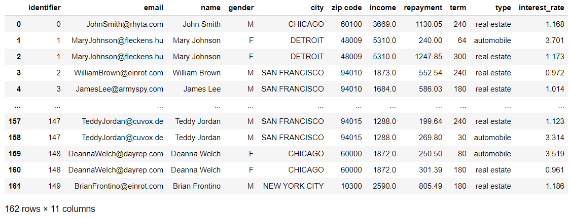
So, there you have it! We now have our amazing DataFrame containing all the informat-- ... Oh, hold on! Wait a second!
Perhaps you didn’t spot it, but we lost some of the loan information when we merged the data. If we look at our loans.csv file, we have 244 loans and their attributes stored in there. However, we only have 162 rows as a result of doing the join. So, where did those other rows go?
There’s one last thing we need to mention about joins that we haven’t already covered, and that’s types of joins. And, in case you hadn’t guessed, it’s due to join types that some of our rows disappeared.
Explore Different Types of Join
When you use Pandas to join data, you really need to specify your join type. The type of join you use will determine how Pandas needs to handle the different keys in our DataFrames, especially if there are matching problems, such as a key present in one DataFrame not being present in the other.
There are four types of joins, which are centered around the various keys:
Inner
Left
Right
Outer
Let’s take a look at each type in detail using the following two DataFrames— height and weight —which contain (yes, you’ve guessed it) the height (in ft/in) and weight (in lbs) of a group of people:
| id | Height |
0 | 1 | 6.0 |
1 | 2 | 5.6 |
2 | 3 | 5.8 |
| id | Weight |
0 | 1 | 175 |
1 | 3 | 165 |
2 | 5 | 155 |
The default type of join is the inner join. Up to now, we’ve only created inner joins. When you do an inner join, the final result of the join will contain only those rows from the first DataFrame that are ALSO present in the second DataFrame.
This means that for each key identified on the right or the left, the process will check for a match in the other table. If a match is found, the key is retained in the results together with the information from the other tables. If a match is not found, this key will not be shown in the final result. The code used for this join is as follows:
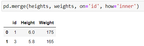
After performing the join, we only have two results, for identifiers 1 and 3. These are the only keys that are present in both tables. 2 is present in the height table but not in weight, while 5 is in weight but not height.
The left join focuses on the identifiers found in the left-hand table (in our case, height). This means that it must retain all keys it finds in the first table and complete the information, wherever possible, with data from the second table.
But what does it do if it can’t find a match?
Well, in that case, in fills in the blanks with missing values. These missing values are defaults, which have no meaning but are used when data is missing. Let’s take a look at the result together to make it clearer:
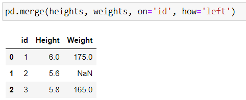
Identifiers 1 and 3 have matches, so they don’t pose any problems. However, identifier 2 only appears in the first DataFrame, so we can’t get the “weight” information for the person who has been assigned identifier 2. The data is missing. Pandas will indicate this using the special value NaN , which is an abbreviation of Not a Number. This is the value Pandas uses to represent any missing data.
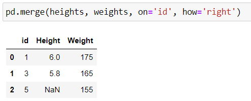
The right join is the alter ego of the left join, but it uses the DataFrame on the right. Here’s the relevant code:
Finally, the outer join is a kind of mash-up of left and right joins. Basically, it means that we keep ALL keys, whether they’re on the left or right, and we fill in the missing information with missing values:
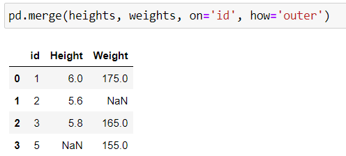
Let’s take a closer look at the result:
Identifiers 1 and 3 have matches, so all information can be displayed.
Identifiers 2 and 5 are only present in one DataFrame (2 is only in height and 5 is only in weight). So, any missing information has been filled in with
NaN.
If we find that some data has disappeared during a join between our customers and loans, this means that some identifiers are not present in one of the two files. In our case, we’re missing information in the customers file which is actually stored in a different file. You could of course do another join, but there’s an alternative solution, and that’s concatenation.
Concatenate Data Using Pandas
Concatenation comes into play when we want to bring together several DataFrames with the same structure in terms of columns and data types, but which contain different data. A typical example would be monthly data exports, where we want to look at the same variables each month (with different values).
And this is also the case for our data. We have two customer files with the same structure, but which contain different data. In this case, we don’t want to join the data, but we want to attach one dataset below the other, as if we’re adding elements to a list using the append method. A join is a horizontal process, whereas concatenation is more vertical.
The Pandas function for concatenating data is concat . If you want to concatenate a number of DataFrames, you just need to put them all into a list and use the concat function on this list.
Here’s an example of how we’d do it with two DataFrames, df1 and df2 :
concat_list = [df1, df2]
pd.concat(concat_list)Let’s now apply everything we’ve learned about these functions and methods to bring the data from our three data files together in the next exercise.
Over to You!

Background
Our data is spread out over multiple files. On one hand, we have the file that contains all of our loan information, which we’ve already used several times. On the other hand, we have all of our customer information, which is held in not one but two files.
It would be really handy to bring this data together into a single file.
Guidelines
This time, your task will be to bring these files together so that you have more options for analyzing and processing the data. You’ll need to use all of the datasets we’ve provided (the two customer files and the loans file) and merge them using the various Pandas methods we’ve covered in this part of the course.
Ready? Let’s get started on this exercise!
Check Your Work
Why don’t you compare your answers with the solution?
Let’s Recap
There are two ways of merging two DataFrames:
If the DataFrames have the same structure, you can concatenate them using the
concat. function to place the DataFrames one after the other.Otherwise, you can join them using the
mergefunction/method.
A join enables you to combine data from two DataFrames using a key, which is a variable present in both DataFrames.
There are four types of joins:
Inner join, which retains any keys that are found in both the first and the second DataFrames.
Right join (or left join), which only retains keys from the right-hand (or left-hand) DataFrame, filling in any missing data using the missing value indicator,
NaN.Outer join, which retains all keys found in EITHER the first OR the second DataFrame.
Now we’re ready to start manipulating the data in our DataFrames. Let’s test out your knowledge with a quiz.
