Identify the Problem of Multicollinearity
Correlation between input features () and our target feature () is a good sign that our input features have predictive power. For example, if we are trying to predict the sales of ice cream, the correlation between hot weather and sales of ice cream can be exploited!
What is Multicollinearity?
Multicollinearity is a subtle problem that can crop up without you noticing.
It describes the situation where features in your input set ( ) are strongly correlated with each other, to the extent that you can predict one input feature from another input feature. Whilst this doesn't generally adversely affect the quality of your model, it can affect your ability to interpret the model. Let's take a look at an example.
Consider a linear regression model that predicts fuel consumption for car journeys to and from work for a group of employees using the following features:
distance travelled
wind speed
average speed
Remember that linear regression works by computing coefficients to plug into a formula for the line of best fit through the data points. So, in this case, we want to come up with a formula of the form:
where m1, m2 and m3 are the coefficients for the respective features and c is the intercept on the y axis.
Let's say the model came up with the following coefficients for the three features:
m1 = 20
m2 = 1
m3 = 2
c = 3
This would give us a linear regression function as follows:
We can see that distance is by far the greatest factor in fuel consumption. For every 1 unit increase in distance we get a 20 unit increase in fuel consumption. The model is easy to interpret.
But what if in the data set the distance was split into "to work" and "from work":
distance travelled to work
distance travelled from work
wind speed
average speed
We would hope that the model would come up with the following linear regression function:
fuel = 10 * distance_to_work + 10 * distance_from_work + 1 * wind - 2 * speed + 3
but it could also come up with different coefficients for the two distance travelled features:
fuel = 7 * distance_to_work + 13 * distance_from_work + 1 * wind - 2 * speed + 3
or
fuel = 15 * distance_to_work + 5 * distance_from_work + 1 * wind - 2 * speed + 3
Consider the following journey parameters:
distance travelled to work = 40
distance travelled from work = 40
wind speed = 5
average speed = 35
Here are the calculations using the above 3 models:
fuel = 10 * 40 + 10 * 40 + 1 * 5 - 2 * 35 + 3 = 735
fuel = 7 * 40 + 13 * 40 + 1 * 5 - 2 * 35 + 3 = 735
fuel = 15 * 40 + 5 * 40 + 1 * 5 - 2 * 35 + 3 = 735
Given the consistency, you may feel that all is good, right? But when it comes to interpreting the models, things get a little tricky. For the first model, we might say that the distance to and from work have equal bearing on fuel consumption because the coefficients are the same. But we would be inclined to interpret the third model as saying that the distance travelled to work is three times as significant as the distance travelled from work. This is clearly not an accurate interpretation.
Spot Multicollinearity
When building models, keep an eye out for features in your input feature set that add no more information that other features in your feature set. For example:
Spot Related Features
If you already have female as a feature you don't also need male as a feature. Why? Because, under the assumption that gender is binary, information about one gender implies information about the other gender:

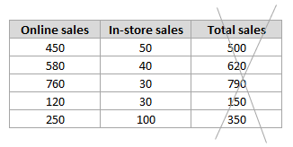
Similarly, if you have features for online sales and in-store sales, you don't need a feature for total sales:
Spot Repeated Features
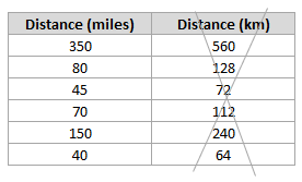
If you have distance in miles and distance in km, remove one of them. Why? Because distance in miles and distance in km give you the same information:
Similarly, if you have temperature in degrees C and temperature in degrees F, remove one of them.
Spot Dummy Variables
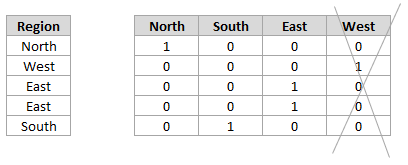
If you have a categorical feature, such as region, which you one-hot-encode (i.e. create dummy variables) you can drop the final column as it adds no additional information (it is essentially encoded by the other columns all being 0):
Spot Highly Correlated Features
Use measures of correlation to understand the correlations between input features.
You can obtain the correlation between features using the following code:
dataset.corr()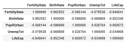
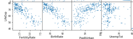
You can plot a scatter matrix using the following code:
pd.plotting.scatter_matrix(dataset, diagonal='kde')
You can display a correlation heatmap using the following code:
def correlationMatrix(df):
    '''Show a correlation matrix for all features.'''
    columns = df.select_dtypes(include=['float64','int64']).columns
    fig = plt.figure(figsize=(10,10))
    ax = fig.add_subplot(111)
    cax = ax.matshow(df.corr(), vmin=-1, vmax=1, interpolation='none',cmap='RdYlBu')
    fig.colorbar(cax)
    ax.set_xticks(np.arange(len(columns)))
    ax.set_yticks(np.arange(len(columns)))
    ax.set_xticklabels(columns, rotation = 90)
    ax.set_yticklabels(columns)
    plt.show()

correlationMatrix(dataset)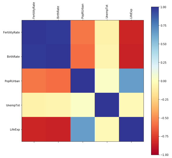
In the above example, if our target feature was LifeExp, we would be encouraged by the high correlation between some of our input features and LifeExp, as shown in the correlation matrix:

and in the scatter plot:
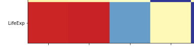
and in the heat map:
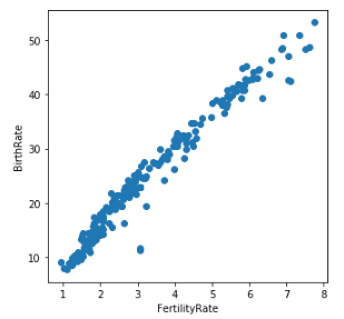
However, we should be concerned about the high level of correlation between some of the input features, in particular, the very strong correlation of 0.98 between FertilityRate and BirthRate:
Reduce Multicollinearity
We can look out for multicollinearity in our input features and manually remove the offending features. Later in the course, we will examine ways to do this more systematically using:
Feature selection
Algorithms that automatically remove features
Summary
Where we have features in the input feature set that are highly correlated with each other, we say we have multicollinearity.
This can lead to situations where our model is difficult to interpret, even though the predictive power of the model is not affected.
Some tell-tale signs of multicollinearity include:
Related features
Repeated features
Highly correlated features
Inclusion of all dummy variables
That's it for the first part! Ready to put your newfound knowledge to the test? Then let's go!
