Evaluate the Performance of a Classification Model
In this chapter, we will explore a number of ways to assess the performance of a classification model. Ready? Excited? Let's go!
The Accuracy Score: Identify It's Limitations
In the previous course, Train a Supervised Machine Learning Model, we evaluated the performance of classification models by computing the accuracy score. We defined the accuracy score as:
accuracy = number of correct predictions / total number of predictions
So, if I had 100 people, 50 of whom were cheese lovers and 50 of who were cheese haters, and I correctly identified 36 of the cheese lovers and 24 of the cheese haters, my accuracy would be
accuracy = (36+24) / (50+50) = 60%.
If I told you that I had built a model that could predict, with over 99% accuracy, whether you would win the lottery or not, would you be impressed?
Whilst accuracy score is fine for balanced classes, like the cheese lovers/haters example above, it can be very misleading for unbalanced classes.
What are balanced and unbalanced classes?
Balanced classes are those where we have an equal number of individuals in each class in our sample. Here is a balanced class:
Cheese lovers: 50 people
Cheese haters: 50 people
Unbalanced classes are those where there are unequal numbers of individuals in each class in our sample. Here is an unbalanced class:
Lottery winners: 1 person
Lottery losers: 45 million people
In the lottery winner prediction example, I can get well over 99% accuracy just by predicting that everyone will lose!
accuracy = (45000000 + 0) / (45000000 + 1) = 99.999998%
So, we need to come up with a better way to measure the performance of our classification models...
Use a Confusion Matrix
The confusion matrix breaks down the classification results, showing a summary of the performance of the predictions against the actuals.
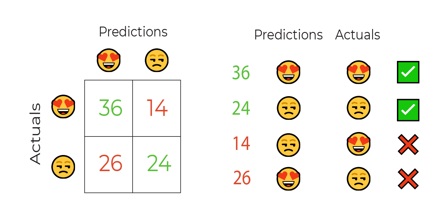
The green cells on the diagonal represent the correct classifications, the white cells represent the incorrect classifications. As you can see, this gives a much more detailed overview of how our model is performing.
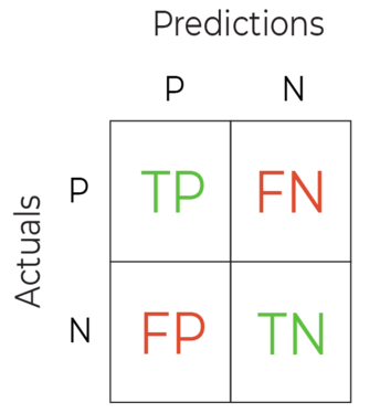
In the general case of a binary classification, we use the following terms for the 4 boxes:
True Positive (TP)
True Negative (TN)
False Positive (FP)
False Negative (FN)
Here they are in their respective boxes:
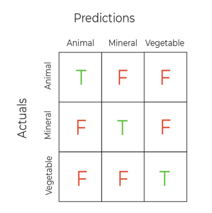
If we have more than two classes, we can extend the confusion matrix accordingly:
The confusion matrix is a really useful device for seeing the detail behind the classification results. But accuracy score has the advantage of being a single number that we can use to compare multiple competing models.
Use Precision / Recall
Imagine you are approached by the owner of an orchard, producing large quantities of apples for different markets. The orchard has two key customers.
One is a supermarket, whose marketing line is “good food at low prices”.
The other is a premium cider manufacturer, whose marketing line is “producing the highest-quality cider from only the finest apples”.
Sometimes bad apples enter the batch, and the orchard has machines with various sensors to identify certain faults in the apples. Color, firmness, blemishes, size, and many other attributes contribute to identifying an apple as bad or good.
You are hired to create two machine learning models. One will try to identify apples suitable for the low-cost supermarket. Let’s call this the SUPERMARKET model. The other will try to identify apples suitable for the premium cider manufacturer. Let’s call this the CIDER model.
So, off you go and build a few models to detect the bad apples based on the tell-tale features. What approach can you use to evaluate and choose the best model for each scenario?
Look at the following two confusion matrices produced by two different models.
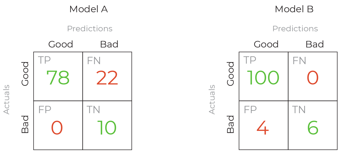
Which is the best for the SUPERMARKET model and which is the best for the CIDER model?
The cost of Model A is that we have some false negatives. In other words, we allow some good apples to be rejected. The cost of Model B is that we have some false positives. In other words, some bad apples slip through into the batch.
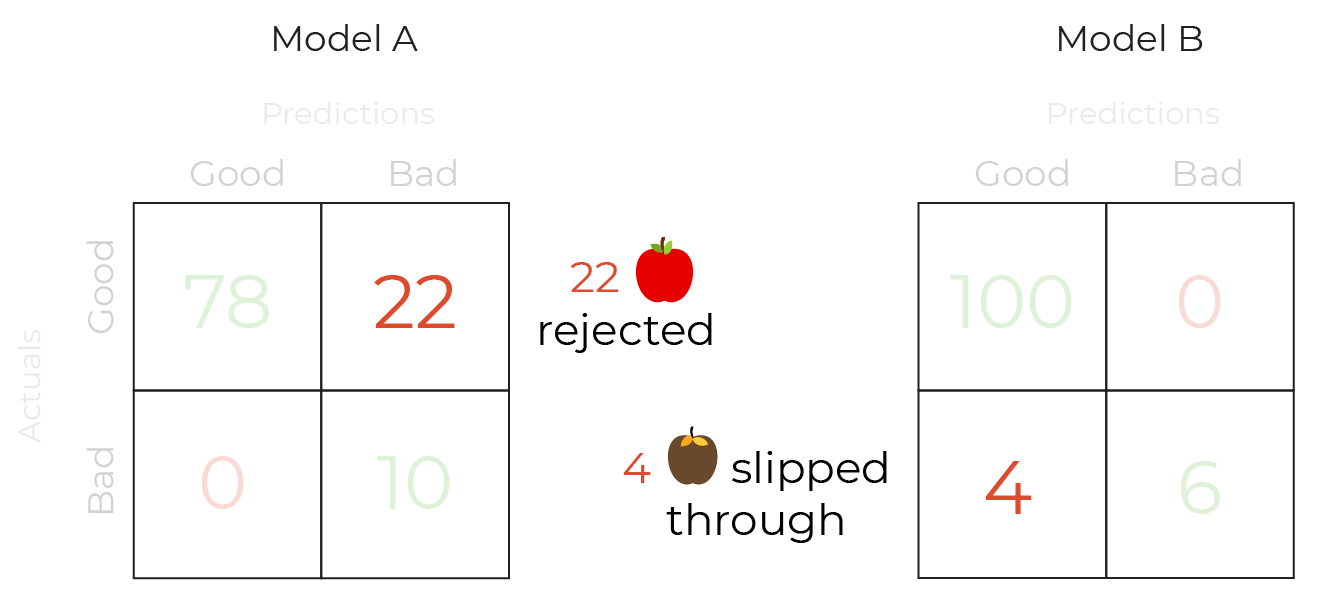
For our CIDER model, which is worse? That we allow 4 bad apples to spoil the whole cider batch (Model B) or that we reject 22 good apples (Model A)? Certainly, we don’t want to spoil the cider! So we would go for model A.
For our SUPERMARKET model, which is worse? That we allow 4 bad apples onto the supermarket shelf (model B), or that we reject 22 good apples (model A)? It would certainly eat into our profits if we kept throwing away so many good apples, so model B would be better.
We can calculate two metrics from the confusion matrix: precision and recall.
Precision is calculated as follows and penalizes models with false positives:
Recall is calculated as follows and penalizes models with false negatives:
Can you calculate precision and recall for our 2 models? Once you are done, check your answers below.
Model A:
Precision = 78 / (78 + 0) = 1
Recall = 78 / (78 + 22) = 0.78
Model B:
Precision = 100 / (100 + 4) = 0.96
Recall = 100 / (100 + 0) = 1
For our SUPERMARKET model, we want to maximize recall. We want to ensure we throw away as few apples as possible. We would favor model B.
For our CIDER model, we want to maximize precision. We want to ensure we don't spoil the batch by processing bad apples. We would favor model A.
Use the F1 score
Having measures to help us pull our models towards high precision or high recall is really useful. But what if we want a balanced measure, one that balances both precision and recall? The F1 score does just that, and is calculated as follows:
Calculating F1 for our two models:
Model A:
F1 = 2 * (1 * 0.75) / (1 + 0.75) = 0.857
Model B:
F1 = 2 * (0.66 * 1) / (0.66 + 1) = 0.795
Use the Receiver Operating Characteristic (ROC) Curve
Some classification algorithms predict a hard in/out classification decision. For example, they may classify an email as spam or not spam.
Other classification algorithms, such as logistic regression, predict a probability that a data point belongs to a specific class. For example, they may say that a particular email is 78% likely to be spam. In this case, we would want to determine a threshold above which we decide an email is spam. We may choose 50%, or perhaps 70%. We can adjust the threshold in order to balance the tradeoff between finding too many false positives or too many false negatives.
But how do we do that? :euh:
A useful evaluation technique would be to examine how a model behaves as this threshold moves. This will give us an idea of how well the model separates the classes. We can then compare different models and see how well each model separates the classes.
For binary classification problems, the Receiver Operating Characteristic curve (ROC curve) provides this technique.
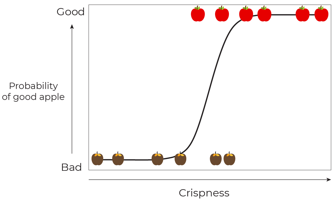
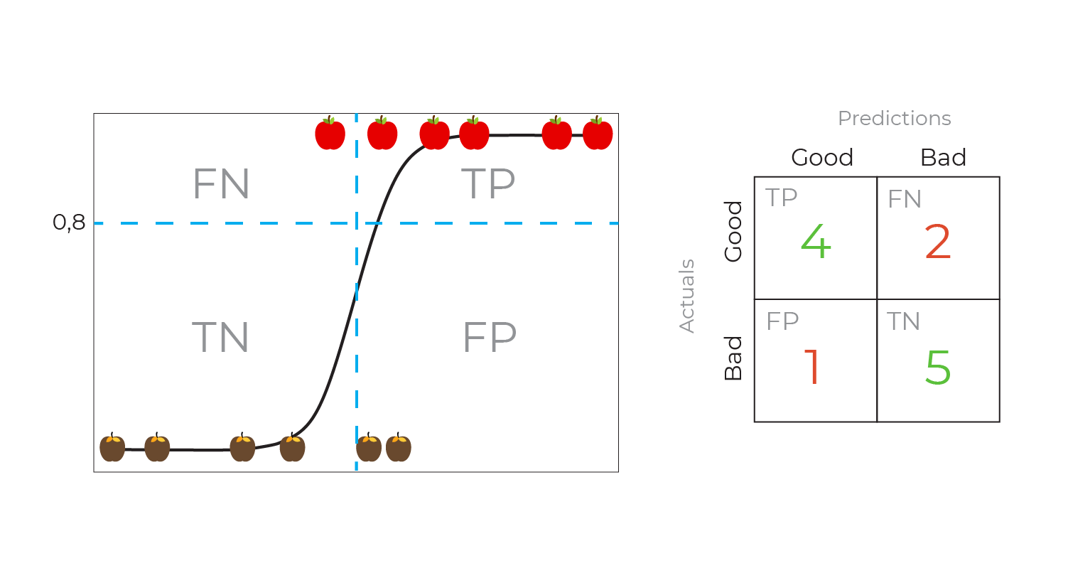
Let's take our apple-selection example from above. We can build a logistic regression model that computes the probability of a good / bad classification based on some feature or set of features (such as crispness of apple). Let's assume we have just 6 good and 6 bad apples:
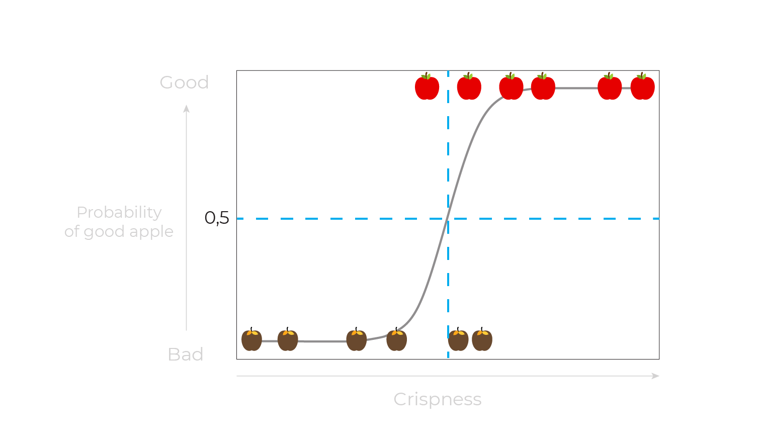
We can set a threshold of 0.5, as shown by the blue dotted lines:
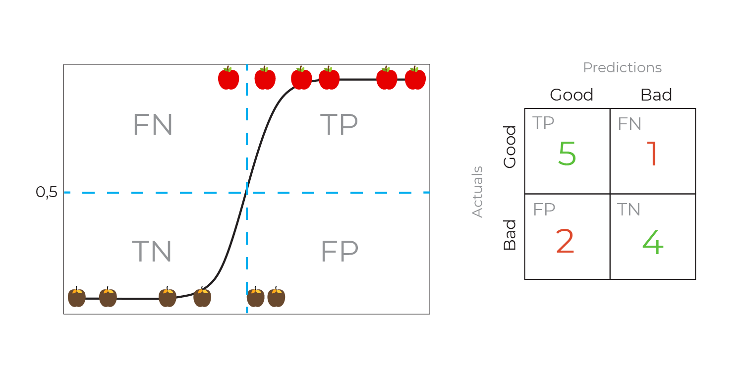
This nicely maps our classification decision onto a confusion matrix, by counting the good and bad apples separated by the blue threshold lines:
If we move the threshold to 0.8, we get a new confusion matrix:
 We can continue in this way, generating confusion matrices for a bunch of different thresholds on the same classification model. We can then compute two new measures from each confusion matrix, the True Positive Rate and False Positive Rate:
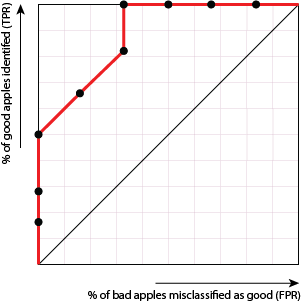
In our example, the TPR is the percentage of good apples found and the FPR is the percentage of bad apples misclassified as good apples. So if we plot TPR against FPR we get a nice view on how well the model behaves as we adjust the threshold and hence how well the model separates the two classes:
If we had another model that produced the following ROC curve, we would conclude that it was less good at separating the good and bad apples:
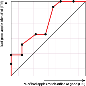
Why is this less good?
Because in order to improve the number of good apples found (i.e. get the dots to move up) we need to suffer more misclassifications of bad apples (i.e. the dots will move to the right).
If, however, we had a model that produced the following ROC curve, we'd have a really excellent model:
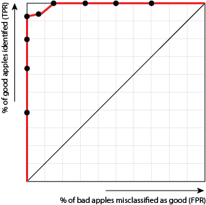
Why is this so good? Because we can increase the number of good apples identified (i..e get the dots to move up) without suffering many more misclassifications of bad apples (i.e. without the dots moving too far to the right).
Use the Area Under the ROC (AUC) Curve
Whilst the ROC curve provides a nice visual representation of the effectiveness of different models, it would be nice to have a single measure to compare the models. We like single measures, don't we? ;) For this, we can compute the area under the ROC curve (called AUC, for "area under curve").
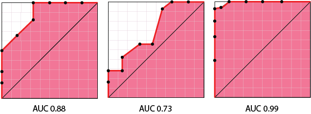
As you can see, the higher the AUC the better the model.
Use Classification Evaluation Metrics with Python
Sklearn makes using these evaluation metrics with your models very straightforward.
A complete example of a model build and evaluation is shown below. It uses Sklearn's built-in breast cancer dataset, which can be used to experiment with building classification models to differentiate between malignant and benign cases. For full details of this (and other) built-in datasets see: https://scikit-learn.org/stable/datasets/index.html.
The Jupyter notebook containing this example code can be found on the course Github repository (see 2.1 Classification Evaluation Metrics.ipynb).
If you need to, refer back to the previous course Train a Supervised Machine Learning Model, for a reminder of the steps in training a supervised model.
First, let's import the functions we need:
# Core libraries
import pandas as pd

# Sklearn processing
from sklearn.preprocessing import MinMaxScaler
from sklearn.model_selection import train_test_split

# Sklearn classification algorithms
from sklearn.tree import DecisionTreeClassifier
from sklearn.linear_model import LogisticRegression

# Sklearn classification model evaluation functions
from sklearn.metrics import classification_report
from sklearn.metrics import accuracy_score
from sklearn.metrics import confusion_matrix
from sklearn.metrics import precision_score
from sklearn.metrics import roc_curve, auc, roc_auc_score

# Matplotlib for charting
import matplotlib.pyplot as plt
Now load the built-in data set:
# Load built-in sample data set
from sklearn.datasets import load_breast_cancer
data = load_breast_cancer()
Let's take a look at the data by converting the built-in data set to a Pandas dataframe:
# View the input features
pd.DataFrame(data.data, columns=data.feature_names).head()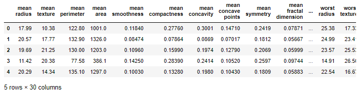
# View the output feature
pd.DataFrame(data.target, columns=["type"]).head()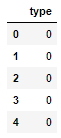
The output features are represented as numbers. Let's see what these numbers represent:
# Check what these output features represent
data.target_names
array(['malignant', 'benign'], dtype='<U9')
So a 0 in the output feature means 'malignant' and a 1 means 'benign'. We have a binary classification task.
Let's select the features to use in our model:
# Define the X (input) and y (target) features
X = data.data
y = data.target
Scale the input features, to avoid problems with variation in the scale of different features.
# Rescale the input features
scaler = MinMaxScaler(feature_range=(0,1))
X = scaler.fit_transform(data.data)
Split the data into training and test sets:
# Split into train (2/3) and test (1/3) sets
test_size = 0.33
seed = 7
X_train, X_test, y_train, y_test = train_test_split(X, y, test_size=test_size, random_state=seed)
Now let's build a logistic regression model. Logistic regression will output a probability for each classification decision.
# Build and fit a logistic regression model
model = LogisticRegression()
model.fit(X_train, y_train)

# Predict the training data
predictions = model.predict(X_train)
We can now plot the confusion matrix for the training set predictions:
# Plot the confusion matrix
print(confusion_matrix(y_train, predictions))
How can you interpret this confusion matrix? Think about the answer then check your answer below.
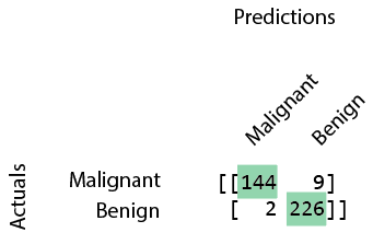
We have 144 cases where we correctly predicted malignant, 226 cases where we correctly predicted benign, 2 cases where we incorrectly predicted malignant instead of benign, and 9 cases where we incorrectly predicted benign instead of malignant.
We can also get the accuracy score for the training set:
# Accuracy score
accuracy_score(y_train, predictions)
0.9711286089238845
Now let's generate a classification report for the training set, which Sklearn uses to summarise the precision, recall and F1 score:
# Classification report
print(classification_report(y_train, predictions, target_names=data.target_names))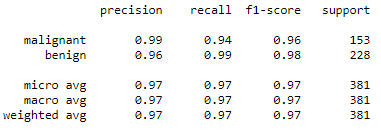
Note that we have the precision, recall and F1 score from the perspective of a malignant classification and the perspective of a benign classification. Looking at just the malignant line, we can see a precision of 0.99 meaning that of the cases where we predict malignant we are correct 99% of the time. We also see a precision of 0.94, meaning that we have correctly found 94% of the malignant cases.
The support column tells us how many data points we have to support the metrics. So we had 153 malignant cases and 228 benign cases in our training set.
Let's now plot the ROC and calculate AUC. I'll define a function for this so we can reuse it whenever we want:
# Define a function to plot the ROC/AUC
def plotRocAuc(model, X, y):

    probabilities = model.predict_proba(X)
    probabilities = probabilities[:, 1]  # keep probabilities for first class only

    # Compute the ROC curve
    fpr, tpr, thresholds = roc_curve(y, probabilities)

    # Plot the "dumb model" line
    plt.plot([0, 1], [0, 1], linestyle='--')

    # Plot the model line
    plt.plot(fpr, tpr, marker='.')
    plt.text(0.75, 0.25, "AUC: " + str(round(roc_auc_score(y, probabilities),2)))

    # show the plot
    plt.show()
And now I can plot the ROC/AUC for the training set:
# ROC / AUC
plotRocAuc(model, X_train, y_train) 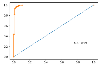
So now we have checked our model performance using the training data, let's properly evaluate it using the test data:
# Evaluate the model
predictions = model.predict(X_test)

print(type(model).__name__)
print("----------------------------------")
print("Confusion matrix:")
print(confusion_matrix(y_test, predictions))

print("\nAccuracy:", accuracy_score(y_test, predictions))

print("\nClassification report:")
print(classification_report(y_test, predictions, target_names=data.target_names))

print("\nROC / AUC:")
plotRocAuc(model, X_test, y_test)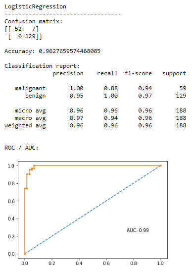
So in terms of identifying malignancy, our model as a high precision (1.0), so we have no false positives, so everyone who is identified as having a malignant cancer really does have malignant cancer.
We have a less impressive recall (0.88), so we have a few false negatives, which are the 7 people who had malignant cancer but were not identified as such.
Wait, what are the lines 'micro avg', 'macro avg' and 'weighted avg' in the classification report?
These are different ways of combining the scores for the malignant line and benign line. I won't explore these any further at this stage, but do investigate them once you are comfortable with using the other techniques covered in this chapter.
Balance Unbalanced Classes
We saw above that unbalanced classes can cause us a few problems. One way to deal with unbalanced classes is to balance them!
Oversampling takes the smaller class and adds copies of a random selection of its data points until the smaller class is the same size as the larger class.
Undersampling takes the larger class and removes some data points at random until the larger class is the same size as the smaller class.
In the breast cancer example above, we have:
228 benign
153 malignant
Oversampling will add 75 random copies of rows from the malignant data, so we end up with:
228 benign
228 malignant
Undersampling will remove 75 rows from the benign data, so we end up with:
153 benign
153 malignant
There are, understandably, downsides to this approach. When oversampling, because we are repeating rows, there is a chance we will overfit our model. When undersampling, because we are removing potentially valuable information, we can end up with underperforming models.
On the course Github repository, you will find a reworking of the above Python code which applies this resampling technique (see 2.1 Classification Evaluation Metrics with Resampling.ipynb).
Here is how we can oversample the malignant cases to balance the classes:
from sklearn.utils import resampleDo our train/test split as usual:
# Split into train (2/3) and test (1/3) sets
test_size = 0.33
seed = 7
X_train, X_test, y_train, y_test = train_test_split(X, y, test_size=test_size, random_state=seed)
Re-combine the X and y training data:
# Put X and y training data back together again
Xy_train = pd.concat([X_train, y_train], axis=1)
Split the training data into its classes:
# Split into malignant and benign
Xy_train_malignant = Xy_train[Xy_train.benign==0]
Xy_train_benign = Xy_train[Xy_train.benign==1]
Find the size of the two classes:
# Count the malignant cases
Xy_train_malignant_count = Xy_train_malignant.shape[0]
Xy_train_malignant_count
153
# Count the benign cases
Xy_train_benign_count = Xy_train_benign.shape[0]
Xy_train_benign_count
228
Oversample the smaller malignant class until it has 228 rows:
# Oversample malignant
Xy_train_malignant_oversampled = resample(Xy_train_malignant, replace=True, n_samples=Xy_train_benign_count)
Recombine the classes, showing that we now have rebalanced classes:
# Combine the two classes
combined = pd.concat([Xy_train_malignant_oversampled, Xy_train_benign])

# Show that we how have balanced classes
combined.benign.value_counts()
1 228
0 228
Resplit the training data into X and y:
# Re-split the training data
y_train = combined.benign
X_train = combined.drop('benign', axis=1)
From this point, we can proceed with building our model as normal.
Summary
Accuracy score tells the percentage of correct predictions we made. As an evaluation measure, it has limitations, particularly when we are dealing with unbalanced classes.
A confusion matrix breaks down the classification results into true positives, true negatives, false positives and false negatives.
Precision is an evaluation measure that penalizes models with false positives. A value of 1 indicates perfect precision.
Recall is an evaluation measure that penalises models with false negatives. A value of 1 indicates perfect recall.
F1 score is an evaluation measure that balances precision and recall. A value of 1 indicates perfect precision and recall.
The ROC curve shows how effectively a model splits binary classes. The best models hug the top left of the chart.
The AUC provides a numerical measure for comparing ROC curves. A value of 1 indicates a model that perfectly separates the classes.
Python does the hard work and calculates these metrics for us from our model outputs.
We can rebalance unbalanced classes using oversampling or undersampling.
In the next chapter, we are going to explore how to evaluate the performance of a regression model.
