Improve the Performance of a Machine Learning Model

So far in this course we have been creating models using the default settings. For example, we can create a KNN regressor in Python by constructing a KNeighborsRegressor with no arguments:

model = KNeighborsRegressor()

We can inspect the model to see what these default settings are:

model

KNeighborsRegressor(algorithm='auto', leaf_size=30, metric='minkowski',metric_params=None, n_jobs=None, n_neighbors=5, p=2, weights='uniform')

We call these settings hyperparameters. 

We can look up the possible values for the hyperparameters of a particular algorithm in the Sklearn documentation. We can also override the default hyperparameters when we create a model:

model = KNeighborsRegressor(n_neighbors=5, weights='distance')

We can guess, but a more systematic approach would be useful. That's where GridSearchCV comes along!

Tune Hyperparameters Using GridSearchCV

Grid search cross-validation builds multiple models using different combinations of hyperparameters and sees which combination performs the best.

We can use the evaluation metrics that we looked at earlier in this course:

• for classification, we can use accuracy score, precision, recall, f1 score or roc-auc,

• for regression, we can use MAE, RMSE or R-squared

Sklearn's GridSearchCV() function does the hard work of building and evaluating models with different combinations of hyperparameters.

For example, if we wanted to use KNeighborsRegressor and wanted to tune the n_neighbors hyperparameter using these candidate values

2, 3, 4, 5, 6

and tune the weights hyperparameter using these candidate values

'uniform','distance'

here is the code we would need. The code assumes we already have our $\$\backslash (X\backslash )\$$ and $\$\backslash (y\; \backslash )\$$ set.

First, we will select our algorithm:

# Select an algorithm
algorithm = KNeighborsRegressor()

We will adopt the approach we saw in the last chapter of using k-fold cross-validation. In this example, I use 3 folds (typically you may use 5 to 10):

# Create 3 folds
seed = 13
kfold = KFold(n_splits=3, shuffle=True, random_state=seed)

Now we can create a set of candidate hyperparameters that we want to examine:

# Define our candidate hyperparameters
hp_candidates = [{'n_neighbors': [2,3,4,5,6], 'weights': ['uniform','distance']}]

And we can pass this algorithm and set of hyperparameters to the GridSearchCV() function, asking it to use R-squared to evaluate the models it creates. We fit each model it creates using the training data:

# Search for best hyperparameters
grid = GridSearchCV(estimator=algorithm, param_grid=hp_candidates, cv=kfold, scoring='r2')
grid.fit(X, y)

Finally, we can inspect the grid and see which combination of model hyperparameters gave us the best R-squared value:

# Get the results
print(grid.best_score_)
print(grid.best_estimator_)
print(grid.best_params_)

0.7664050253839596
KNeighborsRegressor(algorithm='auto', leaf_size=30, metric='minkowski', metric_params=None, n_jobs=None, n_neighbors=3, p=2, weights='distance')
{'n_neighbors': 3, 'weights': 'distance'}

So, GridSearchCV() has determined thatn_neighbors=3 andweights=distance is the best set of hyperparameters to use for this data. Using this set of hyperparameters, we get an evaluation score of 0.77.

In our example above we have 10 unique combinations of hyperparameters (5 candidate values for n_neighbors times 2 candidate values for weights). And for each of those 10 combinations, the 3-fold cross-validation creates 3 models. So in this example, GridSearchCV() creates and evaluates 30 models, as shown in the following diagram:

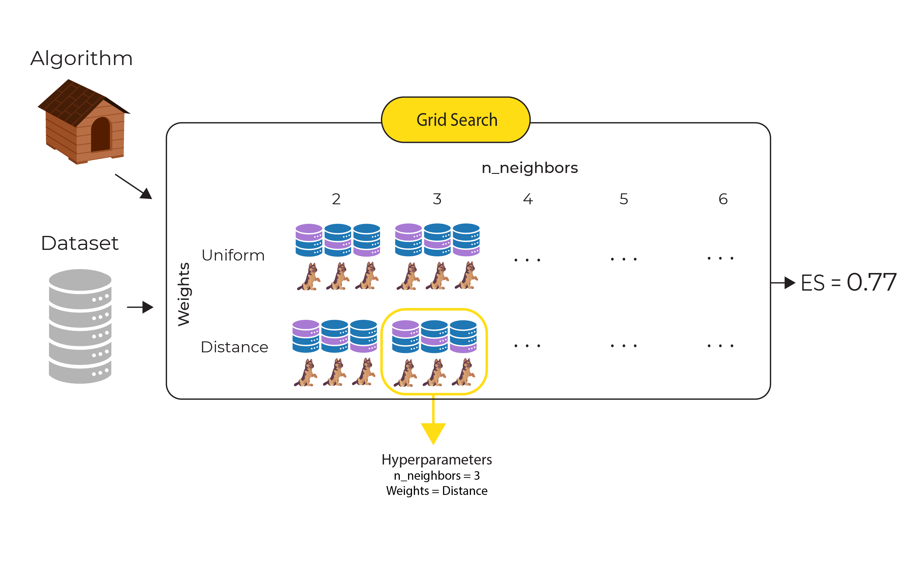
The 3-fold cross-validation for the best combination of hyperparameters (n_neighbors=3 and weights-distance) is circled, and the evaluation score returned (0.77) is the mean of the evaluation scores for these 3 models.

We can get a full breakdown of what GridSearchCV() has done by inspecting the cv_results_ attribute:

grid.cv_results_

We will get back a wealth of information, including the unique hyperparameter combinations that were examined:

'params': [{'n_neighbors': 2, 'weights': 'uniform'},
{'n_neighbors': 2, 'weights': 'distance'},
{'n_neighbors': 3, 'weights': 'uniform'},
{'n_neighbors': 3, 'weights': 'distance'},
{'n_neighbors': 4, 'weights': 'uniform'},
{'n_neighbors': 4, 'weights': 'distance'},
{'n_neighbors': 5, 'weights': 'uniform'},
{'n_neighbors': 5, 'weights': 'distance'},
{'n_neighbors': 6, 'weights': 'uniform'},
{'n_neighbors': 6, 'weights': 'distance'}],

and the 30 R-squared scores, broken down into the 3-fold splits:

'split0_test_score': array([0.75746893, 0.77908312, 0.70347418, 0.76215602, 0.6694333 , 0.74843647, 0.69081694, 0.75488853, 0.6856312 , 0.75527275]),
'split1_test_score': array([0.7563289 , 0.77658452, 0.74134188, 0.77490906, 0.70229635, 0.75883128, 0.69261149, 0.74883153, 0.68249855, 0.73851307]),
'split2_test_score': array([0.74306357, 0.75452132, 0.74565457, 0.77645934, 0.73099167, 0.77635982, 0.7114727 , 0.76799139, 0.68645688, 0.75685882]),

Now we have the best hyperparameters identified by GridSearchCV() we can use them when building our final model.

Take a look at the sample code on the course Github repository for a fully worked example.

Summary

• Hyperparameters are available for each algorithm and allow us to tweak the algorithm behaviour

• The Sklearn function GridSearchCV() can be used to run multiple models in order to select the best combination of hyperparameters for a particular data set.

In the next chapter, we are going to improve regression with regularization!