• 8 hours
  • Hard

Free online content available in this course.

course.header.alt.is_certifying

Got it!

Last updated on 3/8/23

Train a Small Neural Network

Your Task

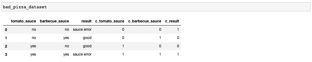
After your astounding success at the factory, you have been asked to help the restaurant franchises. Some restaurant reviewers have complained that they received pizzas with two types of sauce, tomato and barbecue, or no sauce whatsoever. Their pizzas were either too soggy or too dry!

Your data will come from the cameras that sit above the ingredient trays. This will give you information about whether the chef has used - or not - any sauce for the pizza. Here is what the data looks like:


tomato_sauce

barbecue_sauce

result

0

no

no

sauce error

1

no

yes

good

2

yes

no

good

3

yes

yes

sauce error

Understand the Data

Start by putting the data into a pandas DataFrame:

bad_pizza_dataset = pd.DataFrame.from_dict({
        'tomato_sauce': ['no', 'no', 'yes', 'yes'],
        'barbecue_sauce': ['no', 'yes', 'no', 'yes'],
        'result': ['sauce error', 'good', 'good', 'sauce error']
    }
)

And check to see if it looks like in the above table.

Convert the data into numbers again:

bad_pizza_dataset['c_tomato_sauce'] = bad_pizza_dataset['tomato_sauce'].apply(lambda x: 1 if x == 'yes' else 0)
bad_pizza_dataset['c_barbecue_sauce'] = bad_pizza_dataset['barbecue_sauce'].apply(lambda x: 1 if x == 'yes' else 0)
bad_pizza_dataset['c_result'] = bad_pizza_dataset['result'].apply(lambda x: 1 if x == 'sauce error' else 0)

It should look like this now:

A screenshot of the bad pizza dataset used for chapter 2 of the Introduction to Deep Learning course

What does it look like when plotted? 

bad_pizza_dataset.plot(
    kind='scatter',
    x='c_tomato_sauce',
    y='c_barbecue_sauce',
    c='c_result', 
    colormap='jet'
)
Image of the plot that is produced.
Plot Produced by Code

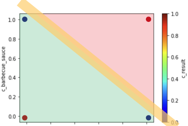
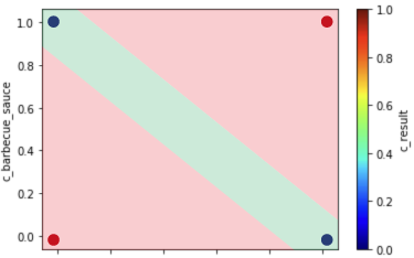
You need one neuron to do one split above the diagonal, producing the red part. However, you can see that the split is not ideal as the green part (the area to the left of the diagonal) contains two blue dots and one red one:

Plot generated from code with an additional diagonal line. There are 3 dots on the left of the line (2 blue and 1 red) and one to the right side (red).
Left = 3 Dots; Right = 1 Dot

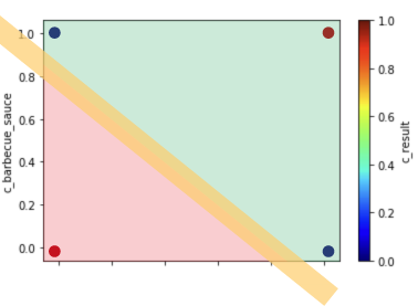
A second neuron would be great to do another split below the diagonal and produce a red part with one red dot (on the left side) and a green part above the split (on the right side) with two blue dots and one red dot.

Plot generated from code with an additional diagonal line. There are 3 dots on the right side of the line (2 blue and 1 red) and one to the left side (red).
Left = 1 Dot; Right = 3 Dots

You can see that both neurons are correct on one side (the one with only 1 dot), but they both make a mistake in their respective other sides.

So if you add one more neuron to help these two decide on their overlap in their respective others sides , you will get something similar to this:

Plot created from code. You need two neurons to create two lines, and then a third to aggregate these results.
A Third Neuron Aggregates The Results

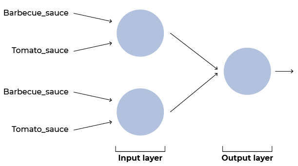
In comparison with the previous chapter, you will only need a different setup for component 1. You will need to build two layers:

  • The input layer will be made of two neurons that can draw two lines, separate the data, and feed this information into the next layer.

  • The output layer will have one neuron that will receive the information from the two neurons before it will output the final result.

Diagram showing the two layers (input and output), as well as the input information (barbecue_sauce and tomato_sauce) to each neuron in the input layer.

This is your first neural network!

Set Up and Train Your First Neural Network

First, set up the layers:

input_layer = Dense(units=2, input_dim=2, activation='sigmoid')

output_layer = Dense(units=1, activation='sigmoid')

Now, the model:

bad_pizza_model = Sequential()
bad_pizza_model.add(input_layer)
bad_pizza_model.add(output_layer)
sgd = SGD()
bad_pizza_model.compile(loss='binary_crossentropy', optimizer=sgd, metrics=[‘accuracy’])

Here’s what it looks like:

bad_pizza_model.summary()

Model: "sequential_1"
_________________________________________________________________
Layer (type)                 Output Shape              Param #   
=================================================================
dense_1 (Dense)              (None, 2)                 6         
_________________________________________________________________
dense_2 (Dense)              (None, 1)                 3         
=================================================================
Total params: 9
Trainable params: 9
Non-trainable params: 0
_________________________________________________________________

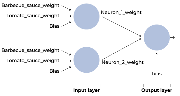
Do you know why there are now nine trainable parameters?

Diagram showing both layers (input and output), as well as the input information to each neuron (barbecue_sauce_weight, tomato_sauce_weight, and bias). The output layer's input is then the weights of both neurons and the bias.

Wait, how are the neurons in the input layer going to discover the error in the output layer? :euh:

Here is where backpropagation comes in. Backpropagation takes the loss from the last layer and propagates it back into the network. Doing so, helps tune the entire network to produce better results - updating the weights across all the neurons in the network.

Let's start training:

history = bad_pizza_model.fit(
    bad_pizza_dataset[['c_tomato_sauce', 'c_barbecue_sauce']], 
    bad_pizza_dataset['c_result'], 
    epochs=3000,
)

The last few epochs show the following:

Epoch 2997/3000
1/1 [==============================] - 0s 974us/step - loss: 0.6829 - accuracy: 0.7500
Epoch 2998/3000
1/1 [==============================] - 0s 947us/step - loss: 0.6829 - accuracy: 0.7500
Epoch 2999/3000
1/1 [==============================] - 0s 921us/step - loss: 0.6829 - accuracy: 0.7500
Epoch 3000/3000
1/1 [==============================] - 0s 893us/step - loss: 0.6829 - accuracy: 0.7500

You want to find out how the model is performing, so let's evaluate it again:

test_loss, test_acc = bad_pizza_model.evaluate(
    bad_pizza_dataset[['c_tomato_sauce', 'c_barbecue_sauce']], 
    bad_pizza_dataset['c_result']
)

print(f"Evaluation result on Test Data : Loss = {test_loss}, accuracy = {test_acc}")

You probably got a result that is not great, like the one below:

1/1 [==============================] - 0s 1ms/step - loss: 0.6829 - accuracy: 0.7500
Evaluation result on test data : Loss = 0.6828916668891907, accuracy = 0.75

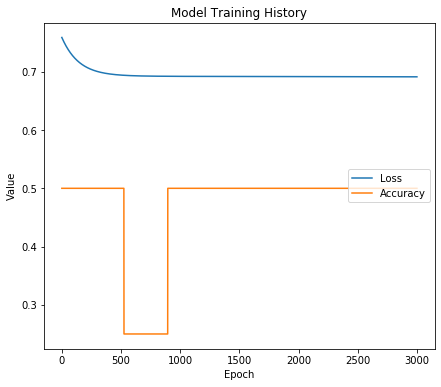
The model finished training, but the results are not as good as expected. To debug it, let's look at how training loss is changing:

plt.figure(figsize=(7, 6))
plt.plot(history.history['loss'])
plt.plot(history.history['accuracy'])
plt.title('Model Training History')
plt.ylabel('Value')
plt.xlabel('Epoch')
plt.legend(['Loss', 'Accuracy'], loc='center right')
plt.show()
Image of the plot resulting from the above code.

Your graph might look a bit different, but here’s how to interpret it: Loss moves slowly down, meaning that the model is learning; however, training is going very slowly - the learning rate could be too small. It could even be stuck. Let's try increasing the learning rate!

input_layer = Dense(units=2, input_dim=2, activation='sigmoid')
output_layer = Dense(units=1, activation='sigmoid')

bad_pizza_model = Sequential()
bad_pizza_model.add(input_layer)
bad_pizza_model.add(output_layer)

high_lr_sgd = SGD(learning_rate=10)

bad_pizza_model.compile(loss='binary_crossentropy', optimizer=high_lr_sgd, metrics=['accuracy'])

bad_pizza_model.summary()

The model looks just like before:

Model: "sequential_2"
_________________________________________________________________
Layer (type)                 Output Shape              Param #   
=================================================================
dense_3 (Dense)              (None, 2)                 6         
_________________________________________________________________
dense_4 (Dense)              (None, 1)                 3         
=================================================================
Total params: 9
Trainable params: 9
Non-trainable params: 0
_________________________________________________________________

Now let’s train:

high_lr_model_history = bad_pizza_model.fit(
    bad_pizza_dataset[['c_tomato_sauce', 'c_barbecue_sauce']], 
    bad_pizza_dataset['c_result'], 
    epochs=3000
)

You probably got similar results:

Epoch 2997/3000
1/1 [==============================] - 0s 2ms/step - loss: 0.3467 - accuracy: 0.5000
Epoch 2998/3000
1/1 [==============================] - 0s 1ms/step - loss: 0.3467 - accuracy: 0.5000
Epoch 2999/3000
1/1 [==============================] - 0s 1ms/step - loss: 0.3467 - accuracy: 0.5000
Epoch 3000/3000
1/1 [==============================] - 0s 1ms/step - loss: 0.3467 - accuracy: 0.5000

They look more promising as the loss is now lower!

Let's quickly check the training loss and see how the session went:

plt.figure(figsize=(7, 6))
plt.plot(high_lr_model_history.history['loss'])
plt.plot(high_lr_model_history.history['accuracy'])
plt.title('Model Training History')
plt.ylabel('Value')
plt.xlabel('Epoch')
plt.legend(['Loss', 'Accuracy'], loc='center right')
plt.show()
Plot output resulting from the code above.

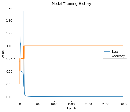
Instead of loss slowly reducing, it increased initially, signifying that the learning rate parameter is too large, which could make loss jump up or get stuck again.

Finally, try a learning rate of 1:

input_layer = Dense(units=3, input_dim=2, activation='sigmoid')
output_layer = Dense(units=1, activation='sigmoid')

bad_pizza_model = Sequential()
bad_pizza_model.add(input_layer)
bad_pizza_model.add(output_layer)

sgd = SGD(learning_rate=1)

bad_pizza_model.compile(loss='binary_crossentropy', optimizer=sgd, metrics=['accuracy'])

bad_pizza_model.summary()

And train it:

history_model = bad_pizza_model.fit(
    bad_pizza_dataset[['c_tomato_sauce', 'c_barbecue_sauce']], 
    bad_pizza_dataset['c_result'], 
    epochs=3000
)

You should see results similar to these:

Epoch 2997/3000
1/1 [==============================] - 0s 1ms/step - loss: 0.0036 - accuracy: 1.0000
Epoch 2998/3000
1/1 [==============================] - 0s 1ms/step - loss: 0.0036 - accuracy: 1.0000
Epoch 2999/3000
1/1 [==============================] - 0s 1ms/step - loss: 0.0036 - accuracy: 1.0000
Epoch 3000/3000
1/1 [==============================] - 0s 1ms/step - loss: 0.0036 - accuracy: 1.0000

Now when you test it:

test_loss, test_acc = bad_pizza_model.evaluate(
    bad_pizza_dataset[['c_tomato_sauce', 'c_barbecue_sauce']], 
    bad_pizza_dataset['c_result']
)

print(f"Evaluation result on Test Data : Loss = {test_loss}, accuracy = {test_acc}")

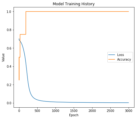
1/1 [==============================] - 0s 1ms/step - loss: 0.0036 - accuracy: 1.0000
Evaluation result on test data: Loss = 0.0036133197136223316, accuracy = 1.0

The model is predicting correctly, and in the chart below, you can see how it finally converged:

plt.figure(figsize=(7, 6))
plt.plot(history_model.history['loss'])
plt.plot(history_model.history['accuracy'])
plt.title('Model Training History')
plt.ylabel('Value')
plt.xlabel('Epoch')
plt.legend(['Loss', 'Accuracy'], loc='center right')
plt.show()
Plot output from the code above.

Do you always need to tune the learning rate?

Let’s Recap!

  • Larger networks can be built by adding more layers. 

  • In larger networks, backpropagation will propagate the error backward across the network to adjust weights in all the neurons and thus tune the network to produce better results.

  • The learning rate parameter can have huge influences on training. Too small of a value will require multiple epochs to train the algorithm, and too large can make the errors higher and even get the algorithm stuck and not capable of learning anything.

You have now trained a neural network with multiple layers. Congratulations! In the next chapter, you will train a multi-output neural network and learn how to set it up!

Example of certificate of achievement