Introduction to Deep Learning Models

Your Task

The restaurant delivery teams would like to choose different color boxes based on the pizza types. When a pizza is vegan, they want to put it in a green box, vegetarian in a yellow box, and meat pizzas in blue boxes.

The cameras above the ovens automatically detect the ingredients, and you need to use that information to suggest what colored box to use.

Understand the Data

The data you will need is here. Let’s read it:

pizza_types = pd.read_csv('datasets/pizza_types.csv', index_col=0)

And inspect it:

pizza_types.head(10)

The last three columns specify the pizza type:

• Vegan

• Vegetarian

• Meat

The rest are your input columns.

pizza_types.shape

5520 examples.

Let's split them into an 80% training dataset and a 20% testing dataset.

training_dataset = pizza_types.sample(frac=0.8)
testing_dataset = pizza_types[~pizza_types.index.isin(training_dataset.index)]

Check to see if the split was done correctly:

training_dataset.shape

(4416, 18)

Returns 4416 rows to train on, perfect.

testing_dataset.shape

(1104, 18)

Returns 1104 rows to test on, great!

Set Up and Train Your First Multi-Output Neural Network

The pizza types should be linearly separable as they either contain animal products, or they don’t. For example, the pizzas have meat (meat), or mozzarella and vegetables (vegetarian), or no animal products (vegan). Let's test that assumption by setting up component one with a single layer with 15 input dimensions and three neurons.

This time let’s use softmax activation. Sigmoid does not ensure the outputs are mutually exclusive. You could have two outputs simultaneously, i.e., a vegan and vegetarian pizza; softmax ensures that the results are mutually exclusive.

pizza_type_model = Sequential()
pizza_type_model.add(Dense(3, input_dim=15, activation='softmax'))

sgd = SGD()

pizza_type_model.compile(loss='categorical_crossentropy', optimizer=sgd, metrics=['accuracy'])

pizza_type_model.summary()

Model: "sequential_4"
_________________________________________________________________
Layer (type)                 Output Shape              Param #
=================================================================
dense_7 (Dense)              (None, 3)                 48
=================================================================
Total params: 48
Trainable params: 48
Non-trainable params: 0
_________________________________________________________________

Split the training set into two, so you can keep an eye on the model's performance on unseen data during training as well:

• A training set

• A validation set

You do that during fitting.

And start training:

history_sgd_pizza_type_model = pizza_type_model.fit(
    training_dataset[['corn', 'olives', 'mushrooms', 'spinach', 'pineapple', 'artichoke', 'chilli', 'pepper', 'onion', 'mozzarella', 'egg', 'pepperoni', 'beef', 'chicken', 'bacon',]],
    training_dataset[['vegan', 'vegetarian', 'meaty']],
    epochs=200,
    validation_split=0.2,
)

You should have an output close to this:

Epoch 197/200
111/111 [==============================] - 0s 3ms/step - loss: 0.0544 - accuracy: 1.0000 - val_loss: 0.0616 - val_accuracy: 1.0000

Epoch 198/200
111/111 [==============================] - 0s 3ms/step - loss: 0.0542 - accuracy: 1.0000 - val_loss: 0.0614 - val_accuracy: 1.0000

Epoch 199/200
111/111 [==============================] - 0s 3ms/step - loss: 0.0540 - accuracy: 1.0000 - val_loss: 0.0611 - val_accuracy: 1.0000

Epoch 200/200
111/111 [==============================] - 0s 3ms/step - loss: 0.0537 - accuracy: 1.0000 - val_loss: 0.0609 - val_accuracy: 1.0000

You can now evaluate the model:

test_loss, test_acc = pizza_type_model.evaluate(
    testing_dataset[['corn', 'olives', 'mushrooms', 'spinach', 'pineapple', 'artichoke', 'chilli', 'pepper', 'onion', 'mozzarella', 'egg', 'pepperoni', 'beef', 'chicken', 'bacon',]],
    testing_dataset[['vegan', 'vegetarian', 'meaty']]
)

print(f"Evaluation result on Test Data : Loss = {test_loss}, accuracy = {test_acc}")

 35/35 [==============================] - 0s 2ms/step - loss: 0.0502 - accuracy: 1.0000
Evaluation result on test data: Loss = 0.050164595246315, accuracy = 1.0

The data was linearly separable and you have now trained a network with multiple output neurons! Awesome!

Try Out a Different Optimizer

In the previous chapter, you discovered that sometimes you need to modify the stochastic gradient descent (SGD) learning rate manually for the network to be able to learn.

Many improvements have been made on top of SGD and several algorithms were derived from it. One such algorithm is adaptive moment estimation (Adam). Whereas SGD maintained its learning rate during the training session, Adam varies it based on how the algorithm is learning, making training much faster. 

To get a feeling for Adam, imagine you are a ball rolling down a mountain. When the hill is steep, you go down fast, and when the hill becomes less steep, you go slower - this is how Adam varies the learning rate.

Let's try Adam and see how it behaves:

from tensorflow.keras.optimizers import Adam

To do that, you will have to modify Component 3 - the optimizer:

pizza_type_model = Sequential()

pizza_type_model.add(Dense(3, input_dim=15, activation='softmax'))

adam = Adam()

pizza_type_model.compile(loss='categorical_crossentropy', optimizer=adam, metrics=['accuracy'])

pizza_type_model.summary()

And start training:

history_adam_pizza_type_model = pizza_type_model.fit(
    training_dataset[['corn', 'olives', 'mushrooms', 'spinach', 'pineapple', 'artichoke', 'chilli', 'pepper', 'onion', 'mozzarella', 'egg', 'pepperoni', 'beef', 'chicken', 'bacon',]],
    training_dataset[['vegan', 'vegetarian', 'meaty']],
    epochs=200,
    validation_split=0.2,
)

Your results should look like this:

Epoch 197/200
111/111 [==============================] - 0s 3ms/step - loss: 2.2862e-04 - accuracy: 1.0000 - val_loss: 2.5416e-04 - val_accuracy: 1.0000

Epoch 198/200
111/111 [==============================] - 0s 3ms/step - loss: 2.2079e-04 - accuracy: 1.0000 - val_loss: 2.4536e-04 - val_accuracy: 1.0000

Epoch 199/200
111/111 [==============================] - 0s 3ms/step - loss: 2.1321e-04 - accuracy: 1.0000 - val_loss: 2.3729e-04 - val_accuracy: 1.0000

Epoch 200/200
111/111 [==============================] - 0s 3ms/step - loss: 2.0585e-04 - accuracy: 1.0000 - val_loss: 2.2876e-04 - val_accuracy: 1.0000

Let's compare the training history when using SGD and Adam:

fig, axes = plt.subplots(1, 2, figsize=(14, 6))

axes = axes.flatten()

axes[0].plot(history_sgd_pizza_type_model.history['loss'])
axes[0].plot(history_sgd_pizza_type_model.history['accuracy'])
axes[0].set_title('SGD based Model Training History')
axes[0].set_ylabel('Value')
axes[0].set_xlabel('Epoch')
axes[0].legend(['Loss', 'Accuracy'], loc='center right')
axes[1].plot(history_adam_pizza_type_model.history['loss'])
axes[1].plot(history_adam_pizza_type_model.history['accuracy'])
axes[1].set_title('Adam based Model Training History')
axes[1].set_ylabel('Value')
axes[1].set_xlabel('Epoch')
axes[1].legend(['Loss', 'Accuracy'], loc='center right')
plt.show()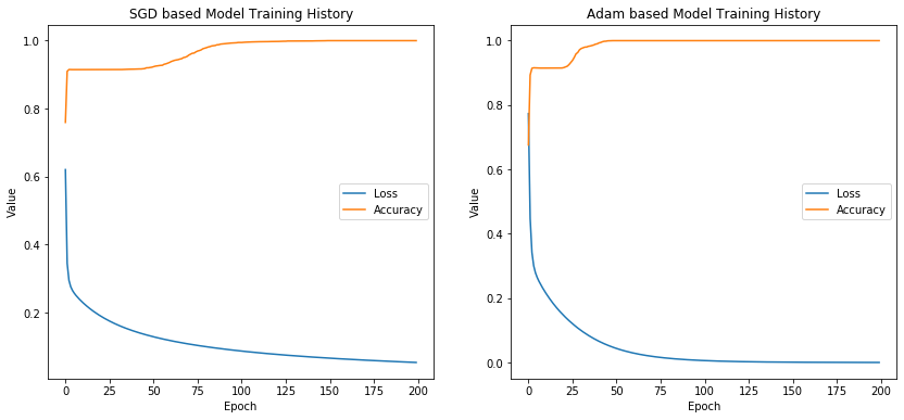

Adam can help you train faster; however, some research suggests that it might tend to push networks into overfitting. Nonetheless, you will still see it widely-used as the go-to algorithm in the industry.

Let’s Recap!

• Stochastic gradient descent is an excellent algorithm for optimization. A great alternative is adaptive momentum estimation (Adam), as it can adjust the learning rate during training.

• Binary cross-entropy helps in situations where the network has one output neuron and needs to decide between binary results such as 0 or 1 as it penalizes the model when the result is different from the expected result. 

• You should use categorical cross-entropy when you have multiple outputs and softmax for activation if the outputs are mutually exclusive.

You have now trained a multi-output neural network. You are ready to build more complex networks!