Train a Deeper Fully Connected Neural Network

Your Task
Your fame meets no bounds at Worldwide Pizza Co.! Teams from around the world reach out for your help. You have received traffic data from one of the restaurant teams. They want to automatically increase delivery times if an order is placed during heavy traffic times.
They asked you to help out and sent you a dataset they recorded with the day, hour, minute, and second their driver recorded as well whether there was any traffic.
Understand the Data
Download the data from here and load it:
traffic_data = pd.read_csv('datasets/traffic_data.csv', index_col=0)And inspect it:
traffic_data.head()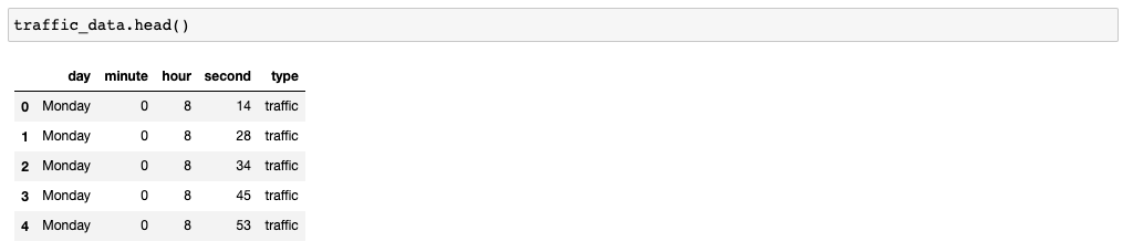
traffic_data.shape()85638 rows. There is a ton of data here! Great! Let's look at the traffic vs. non-traffic variable:
traffic_data['type'].value_counts()no_traffic 50769
traffic 34869
Name: type, dtype: int64
The dataset is imbalanced; there is more data when there is no traffic, but you will manage!
traffic_data['day'].value_counts()Sunday 12278
Saturday 12251
Thursday 12241
Wednesday 12237
Tuesday 12217
Monday 12212
Friday 12202
Name: day, dtype: int64
There is a relatively equal representation of data every day. How about the traffic vs. non-traffic variable per day?
traffic_data.groupby('day')['type'].value_counts()day type
Friday traffic 6989
no_traffic 5213
Monday traffic 6972
no_traffic 5240
Saturday no_traffic 12251
Sunday no_traffic 12278
Thursday traffic 6965
no_traffic 5276
Tuesday traffic 6990
no_traffic 5227
Wednesday traffic 6953
no_traffic 5284
Name: type, dtype: int64
There is a relatively equal traffic vs. no-traffic representation besides Saturdays and Sundays. What about per hour?
traffic_data['hour'].value_counts()8 6211
16 6204
20 6195
18 6188
14 6180
10 6156
12 6147
15 6110
17 6076
13 6052
21 6046
11 6046
19 6036
9 5988
22 3
Name: hour, dtype: int64
Hours start at 8 and stop at 22. 22 has very little data.
Set up the type as a number:
traffic_data['c_type'] = traffic_data['type'].apply(lambda x: 1 if x == 'traffic' else 0)It's quite hard to visualize the data. Nonetheless, let's try to plot days, hours, and type:
import matplotlib.pyplot as plt

from matplotlib.pyplot import colorbar, figure

figure(num=None, figsize=(12, 10))

plt.scatter(
    traffic_data['day'],
    traffic_data['hour'],
    c=traffic_data['c_type'],
    cmap='jet',
)

cbar = colorbar()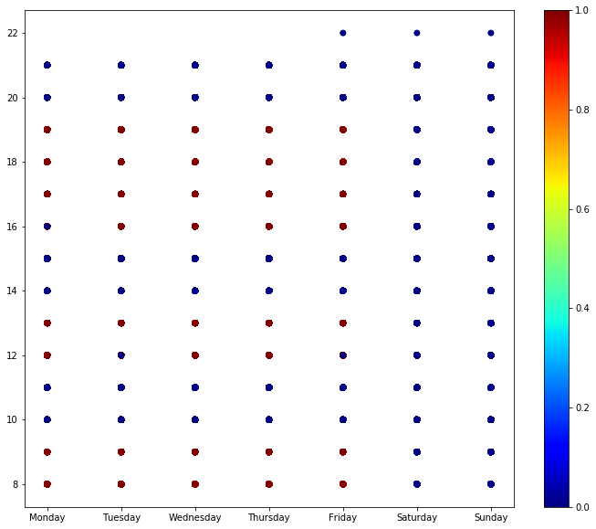
As seen before, there is no traffic on Saturdays or Sundays. It seems to be mostly around some key hours, such as 8-10, 12-13, and 16-20.
Let's first convert the days to new columns using one-hot encoding:
traffic_data = traffic_data.join(pd.get_dummies(traffic_data['day']))Split the data again into a training and test set:
training_dataset = traffic_data.sample(frac=0.8)
testing_dataset = traffic_data[~traffic_data.index.isin(training_dataset.index)]
And select the input columns you will be using from this dataset:
input_columns = [
    'Monday',
    'Tuesday',
    'Wednesday',
    'Thursday',
    'Friday',
    'Saturday',
    'Sunday',
    'hour',
    'minute',
    'second'
]Set Up Your First Neural Network With a Hidden Layer
Let's start setting up the network.
The modifications you need to make are in Component 1. You have to build a network with more layers, as the function that needs to fit this data is now more complex.
A few lines could separate the data in earlier tasks, and it was easy to tell how many neurons you would need. Now you need a more complex shape to separate the two groups - traffic and not traffic.
As a starting point, use three layers with 50 neurons in the input and hidden layer, and just one in the output layer. If you find it works, you can try to reduce that number and see what happens. If it doesn't work, you can always try to increase it.
There are two more changes to make: one, to the activation function, and the second, to the dropout rate.
Change the Activation Function
Change the activation function of the input and hidden layers to use a rectified linear unit (ReLU), which has the following shape:
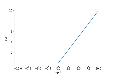
Use this function because deep neural networks can suffer from a phenomenon called gradient vanishing.
Gradient vanishing is a phenomenon that happens when the error that backpropagation pushes back throughout the network gets smaller and smaller as it moves from right to left (output layer towards input layer). That means that the weights of neurons in the first layers end up being updated by minimal values. When this happens, the weights take too long to get to the required value, and the network takes a lot longer to learn.
Because you don't know the size of the network you need and wish to avoid overfitting. You can also use Dropout.
Change the Dropout Rate
As you remember, training a neural network consists of two steps: a forward pass and a backward pass.
When you add dropout to a layer on the forward pass, a fraction of the neurons don't activate, and the next layer receives a 0 value instead of the neuron's result. On the backward pass, the same neurons that ended up not activating also don't get their weights updated. They are basically frozen in that epoch. You can even imagine this as them being effectively cut out from the network like in the graphic below:
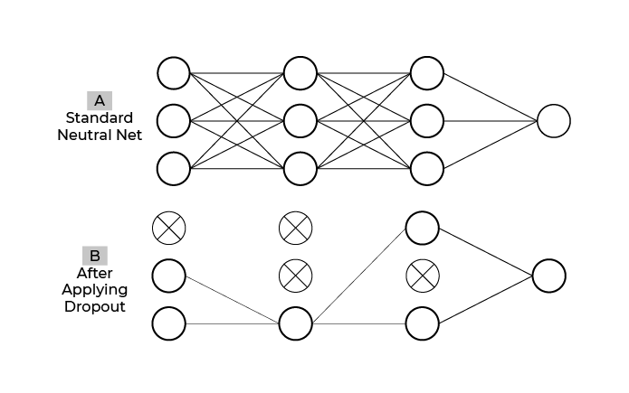
In large networks, neurons start being reliant on certain preceding neurons that end up hindering learning. By employing dropout, those preceding neurons are randomly dropped, which breaks the formed dependency.
Research shows that the best dropout rate is 50%; however, you should start small as dropout can stop a network from learning. I recommend you use a 10% dropout rate here, but you should try larger numbers of neurons and higher dropouts and see how the network behaves during training:
from tensorflow.keras.layers import Dropout

traffic_model = Sequential([
    Dense(32, input_dim=len(input_columns), activation='relu'),
    Dropout(0.1),
    Dense(32, activation='relu'),
    Dropout(0.1),
    Dense(1, activation='sigmoid'),
])

adam = Adam()

traffic_model.compile(loss='binary_crossentropy', optimizer='adam', metrics=['accuracy'])

traffic_model.summary()
And now your summary shows you this:
Model: "sequential"
_________________________________________________________________
Layer (type) Output Shape Param #
=================================================================
dense (Dense) (None, 32) 352
_________________________________________________________________
dropout (Dropout) (None, 32) 0
_________________________________________________________________
dense_1 (Dense) (None, 32) 1056
_________________________________________________________________
dropout_1 (Dropout) (None, 32) 0
_________________________________________________________________
dense_2 (Dense) (None, 1) 33
=================================================================
Total params: 1,441
Trainable params: 1,441
Non-trainable params: 0
_________________________________________________________________
Set Up a Batch Size
This time around also set up a batch size of 100. The batch size represents how many examples the algorithm predicts during training before the weights get updated. At the time of writing this course, Keras had a default batch size of 32:
batch_size = 100When the batch size is greater than one, stochastic gradient descent is normally referred to as mini-batch gradient descent. The parameter does have an impact on training time with larger batches making it faster to train, but large batches have also been shown to make it harder for the algorithm to generalize. A good rule of thumb is to ensure the batch fits into the memory.
history_traffic_model = traffic_model.fit(
    training_dataset[input_columns],
    training_dataset[['c_type']],
    epochs=30,
    validation_split=0.1,
    batch_size=batch_size
)
Epoch 27/30
617/617 [==============================] - 2s 3ms/step - loss: 0.2278 - accuracy: 0.8801 - val_loss: 0.3070 - val_accuracy: 0.8415Epoch 28/30
617/617 [==============================] - 2s 3ms/step - loss: 0.2102 - accuracy: 0.8907 - val_loss: 0.1686 - val_accuracy: 0.9801Epoch 29/30
617/617 [==============================] - 2s 3ms/step - loss: 0.2092 - accuracy: 0.9241 - val_loss: 0.1836 - val_accuracy: 0.9622Epoch 30/30
617/617 [==============================] - 2s 3ms/step - loss: 0.1720 - accuracy: 0.9482 - val_loss: 0.0892 - val_accuracy: 0.9990
When evaluating, you get:
test_loss, test_acc = traffic_model.evaluate(
    testing_dataset[input_columns],
    testing_dataset['c_type']
)

print(f"Evaluation result on Test Data : Loss = {test_loss}, accuracy = {test_acc}")
536/536 [==============================] - 1s 2ms/step - loss: 0.0918 - accuracy: 0.9989
Evaluation result on test data : Loss = 0.09181016683578491, accuracy = 0.9988906979560852
The restaurant team is thrilled with your results!
That’s awesome! You just built your first deep neural network and trained it to a high accuracy. Congratulations!
Let’s Recap!
Rectified linear units are one type of activation function that allows you to deal with the error becoming too small as backpropagation pushes it back through the network during training - a phenomenon also known as gradient vanishing.
Batch sizes allow you to present the algorithm with multiple examples before calculating the loss and updating weights. People typically refer to this as mini-batch gradient descent.
Dropout randomly selects some neurons to skip during training to prevent overfitting.
Congratulations! You have now successfully trained your first neural networks. You are now ready for the test, and after that, in the next part, you will learn more complex networks.
