Introduction to Deep Learning Models

Your Task

Worldwide Pizza Co.'s packaging is legendary. It's the only pizza company that has different shapes of boxes, depending on your order. A 5-piece wings meal comes in a star-shaped box; fries come in a circle-shaped box, and mozzarella sticks in a triangle one.

For now, the box-manufacturing company manually sorts the boxes. They saw that you were featured in a recent company newsletter about AI-solutions and have reached out for your help. They have some cameras on the production line and have sent you pictures of the boxes that they produce. Here are the four types:

• Stars

• Circles

• Squares

• Triangles

They said that they could install a system to automatically push boxes in the right direction if you could create a solution that can successfully detect them. Ready to work your magic? :magicien:

Understand the Data

Your new task involves using image data. Keras already has built-in helper functions that allow you to read the images so you'll use that automatically:

from tensorflow.keras.preprocessing.image import ImageDataGenerator

Download the data from here and save its location in a variable:

working_dir = 'datasets/shapes'

And the box classes:

classes = ['circle', 'square', 'star', 'triangle']

The ImageDataGenerator is a Python generator that automatically gives you more data as you loop through it. Set it up such that you keep 20% of the data for validation:

data_generator = ImageDataGenerator(validation_split=0.2)

And now set its parameters:

training_generator = data_generator.flow_from_directory(
    working_dir, 
    classes=classes, 
    batch_size=100,
    subset='training',
    color_mode='grayscale'
)

Found 11981 images belonging to four classes.

validation_generator = data_generator.flow_from_directory(
    working_dir, 
    classes=classes, 
    batch_size=100,
    subset='validation',
    color_mode='grayscale'
)

Found 2994 images belonging to four classes.

Now check the images to see what they look like:

import matplotlib.pyplot as plt

images, labels = training_generator.next()

fig, axes = plt.subplots(1, 4, figsize=(20,20))

axes = axes.flatten()
axes_idx = 0

for one_hot_label in range(4):
    for image, label in zip(images, labels):
        if label[one_hot_label] == 1:
            ax = axes[axes_idx]
            ax.imshow(image[:,:,0], cmap='Greys_r')
            ax.axis('off')
            ax.set_title(classes[one_hot_label])
            axes_idx += 1
            break
            

plt.tight_layout()

plt.show()

Select one and let's take a look:

first_image_in_batch = images[0]

Here's its shape:

image_shape = first_image_in_batch.shape

print(image_shape)

(256, 256, 1) 

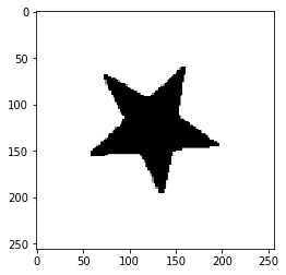
It has 256 pixels x 256 pixels. We can also see that when we plot it:

plt.imshow(first_image_in_batch[:,:,0], cmap='Greys_r')

Inside the machine, the image was read in a single table of 256 rows and 256 columns. Values are stored between 0 and 255. 0 is typically black, and 255 is white. Take a look:

print(first_image_in_batch[:,:,0])

[[255. 255. 255. ... 255. 255. 255.]
[255. 255. 255. ... 255. 255. 255.]
[255. 255. 255. ... 255. 255. 255.]

...

[255. 255. 255. ... 255. 255. 255.]
[255. 255. 255. ... 255. 255. 255.]
[255. 255. 255. ... 255. 255. 255.]]

Printed above are only the edges which we know are white - this is the reason why they have the value 255.

Set Up Your First Convolutional Neural Network

Start by importing a convolutional layer - Conv2D from keras.layers:

from keras.layers import Conv2D

Even small filters have proven to be very powerful at extracting information such as lines, so you use a filter of 5 by 5 and ReLU activation. Add 16 of them:

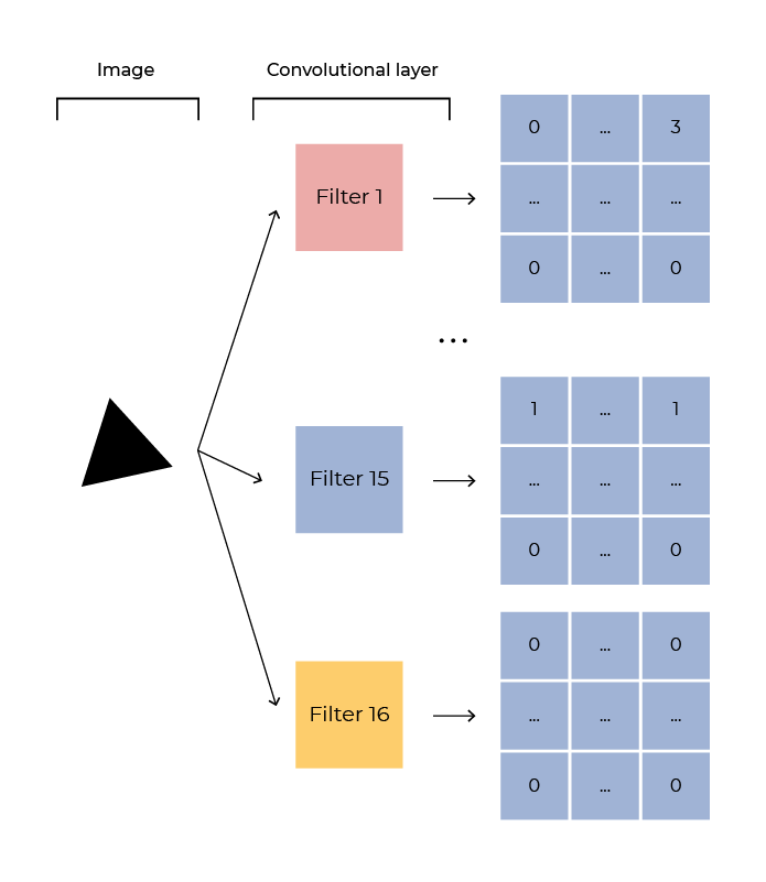
convolutional_layer = Conv2D(16, (5, 5), activation='relu', input_shape=image_shape)

The above setup with 16 filters means you now have 16 sheets where marking is done. The original image size is 256x256, and using a filter of size 5x5 means the filter's resulting image/table size is 252 by 252. The math is not super crazy:

Resulting image size = (number of rows in the image) - (number of rows in the filter - 1).
256 - 5 + 1 = 252

Reduce the sizes of these resulting images by using a max pooling filter:

from keras.layers import MaxPool2D

max_pool_layer = MaxPool2D()

Your convolutional layers have now captured information from neighboring pixels, and your pooling layers have downsampled that data. You can now flatten the results of the max pool layer into a single vector.

from keras.layers import Flatten

flatten_layer = Flatten()

Create a dense layer to receive the flattened data and act as the output. Use softmax as activation for the final layer as you have multiple mutually exclusive outputs:

from keras.layers import Dense

dense_layer = Dense(4, activation='softmax')

Finally, build the model:

from keras.models import Sequential

cnn_model = Sequential([
    convolutional_layer,
    max_pool_layer,
    flatten_layer,
    dense_layer
])


cnn_model.summary()

Model: "sequential_1"
_________________________________________________________________
Layer (type)                 Output Shape              Param #
=================================================================
conv2d_1 (Conv2D)            (None, 252, 252, 16)      416
_________________________________________________________________
max_pooling2d_1 (MaxPooling2 (None, 126, 126, 16)      0
_________________________________________________________________
flatten_1 (Flatten)          (None, 254016)            0
_________________________________________________________________
dense_1 (Dense)              (None, 4)                 1016068
=================================================================
Total params: 1,016,484
Trainable params: 1,016,484
Non-trainable params: 0
_________________________________________________________________

Below is what your model looks like:

There are approximately 1 million parameters to train now. Most of these are in the output layer as it needs to process the results from the flatten layer.

It is quite common for models to have multiple convolutional layers and max pooling layers before the final flatten and dense layer, which reduces the number of parameters that need training. This setup, however, will be enough here.

You can now start training:

cnn_model.compile(
    optimizer='adam',
    loss='categorical_crossentropy',
    metrics=['accuracy'],
)

history = cnn_model.fit(training_generator, epochs=5)

Epoch 1/5
120/120 [==============================] - 11s 91ms/step - loss: 786.0164 - accuracy: 0.8513

Epoch 2/5
120/120 [==============================] - 10s 80ms/step - loss: 0.2239 - accuracy: 0.9978

Epoch 3/5
120/120 [==============================] - 10s 81ms/step - loss: 0.0526 - accuracy: 0.9992

Epoch 4/5
120/120 [==============================] - 10s 81ms/step - loss: 0.0206 - accuracy: 0.9994

Epoch 5/5
120/120 [==============================] - 10s 80ms/step - loss: 5.4657e-06 - accuracy: 1.0000

And once you are done, try it out:

val_loss, val_acc = cnn_model.evaluate(validation_generator)

print(f"Evaluation result on Test Data : Loss = {val_loss}, accuracy = {val_acc}")

30/30 [==============================] - 2s 51ms/step
Evaluation result on test data : Loss = 0.0, accuracy = 0.9983299970626831

Awesome results! Congratulations on building your first CNN! The factory team is very impressed with your work!

Let’s Recap!

• Keras has built-in functionality to deal with images, such as reading them from a directory and splitting them into training/validation datasets: ImageDataGenerator.

• Conv2D, MaxPool2D, and Flatten layers are commonly used to build CNNs in Keras.

• Repeating groups of Conv2D and MaxPool2D layers will initially break down the input image into simpler shapes that will be used by later layers to detect more complex ones.

You are now ready to learn a new type of neural network - recurrent neural networks!