Calculate the Value Spread in your Data
This chapter contains mathematical formulas, but don’t let that scare you! They will be explained step-by-step.
In the last chapter, your friend gave you an estimate of how long your trip should take. But he gave you measures of central tendency, such as, for example, the Mean, which in this case was 60 minutes per trip.
What you need to know now is whether the durations of your friend’s trips “tightly clustered” around 60 minutes (for example: [58, 60, 62, 59, 57...]), or whether they were more loosely dispersed (example: [40, 70, 78, 43, .etc.]).
Why?
If the values tightly cluster around 60 minutes, then you want to leave 75 minutes in advance. That way, you will be likely to arrive 5 or 10 minutes before your interview. But if the values are very far apart, you should leave 100 minutes in advance of your interview, because it’s entirely possible for the trip to take 80 minutes!
I get it! Calculating the value spread... I’m guessing there’s a statistical measure for that?
Absolutely! There are even several. They are called measures of dispersion.
Thinking It Through...
Let’s try to create our own indicator of dispersion, step-by-step. To illustrate it, we’ll use the following values (70, 60, 50, 55, 55, 65, 65), and give each of them a name: , with taking values from 1 to 7. So our value names will run from to .
Formally, this is expressed: , with .
Note that the mean of these values is 60, which is written , and pronounced “x bar.”
Measures of dispersion are easy! Let’s take all of our values and calculate the deviation from the mean for each of them. Then we will add up all of the deviations.
That’s a good start. Because our mean is 60, the deviations of from the mean are: . Except, if we add them all up, we get 0! We can demonstrate this mathematically: no matter how dispersed your values, the sum of the deviations from the mean will always be 0. Not very helpful...
It’s 0 only because there are positive and negative numbers. Let’s get around that by squaring them all. A square number is always positive isn’t it?
That’s right! When we do that, here’s what we get: . Now if we add up all of these values, we get 300.
Okay. But there’s another problem. Here we have 7 values, simply because we are a little bit lazy and only collected 7. But in statistics, the more we collect, the better an idea we have of what we are describing. So we should have collected 10, 100 or even 1,000 values!
However, with 1,000 values, our measure would explode! It would go from 300, with 7 values, to perhaps 40,000,000,000, with 1,000 values. That’s a problem.
So, instead of calculating the sum and blowing up our indicator, let’s take the mean. Whether there are 7 values or 1,000, the mean will not explode.
Good idea. The mean of (100,0,100,25,25,25,25) is 42.86.
Measures of Dispersion
Empirical Variance
Guess what! The indicator we just made is one of the mostly used common indicators in statistics! It’s called the Empirical Variance.
As we just saw, it is equal to
To go further into the calculations aspect, go to the Take It Further section at the end of the chapter. You will also see a “corrected” version of the Empirical Variance referred to as unbiased. For this I also refer you to the Take It Further section. :magicien:
Standard Deviation
The standard deviation is simply the square root of the variance. It is often abbreviated std. In fact, when we calculate the empirical variance of our trip times, the result is expressed in a unit of minutes , which is not very intelligible. If we take the square root, the unit becomes the minute. Here, our standard deviation is 6.55 minutes. It is written
But a standard deviation of 6.55 minutes for a trip of 1 hour (on average) is not the same as a standard deviation of 6.55 minutes for a trip of 24 hours (on average)! This is called a coefficient of variation, which you will find in the Take It Further section.
Inter-Quartile Range
Remember the Median? It’s the “middle” value dividing the higher and lower values.
A quartile is the same thing, except the values are divided by quarters. So there are three quartiles, written (first quartile), (second quartile) and (third quartile). It works like this:
• 1/4 of the values are below , 3/4 are above.
• 2/4 of the values are below , 2/4 are above ( is the Median!).
• 3/4 the values are below , 1/4 are above.
The Inter-Quartile Range is the difference between the 3rd quartile and the 1st quartile:
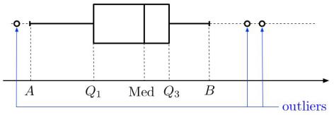
Box-and-Whisker Plots (Box plots)
A box plot is a way of graphically representing groups of numerical data through their quartiles, to indicate the degree of dispersion in the data. and determine the sides of the box, and the median is often indicated inside. Lines (the “whiskers”) then extend vertically from the box to indicate the lowest and highest values...provided that these lines (on either side of the box) are within 1.5 IQR of the upper and lower quartiles of the inter-quartile range. Values below or above are considered outliers; they are not included in the whisker:
Now for the code...
For the empirical variance and the standard deviation, the same principle applies as in the last chapter: we call the var() and std() methods for the variable we are looking at. Full disclosure: these two methods will return results that vary somewhat from those you get with the above data formulas. This gets us into “biased estimators” (for this, the more motivated among us can refer to the section Take It Further: Empirical Variance). To obtain the results described above, we need to add ddof=0 (lines 8 and 9).
We will display the box plots with the histograms, so you can compare :). On line 12, the keyword vert=False is there because we don’t want the box plot to be vertical (we want it to be horizontal!). Taking the code from our previous chapter, here’s what we get:
for cat in data["categ"].unique():
    subset = data[data.categ == cat] # Creation of sub-sample
    print("-"*20)
    print(cat)
    print("mean:\n",subset['amount'].mean())
    print("med:\n",subset['amount'].median())
    print("mod:\n",subset['amount'].mode())
    print("var:\n",subset['amount'].var(ddof=0))
    print("ect:\n",subset['amount'].std(ddof=0))
    subset["amount"].hist() # Creates the histogram
    plt.show()  # Displays the histogram
    subset.boxplot(column="amount", vert=False)
    plt.show()
The variance of the transaction amount for the RENT category is null, meaning the rent amount is always the same.
Take It Further: The Corrected Empirical Variance
The best way of estimating the variance of a random variable (i.e., the theoretical variance) is not the Empirical Variance.
Surprising, no? Yes. When we get deep into the calculations, we see that the empirical variance gives values that are lower (on average) than the variance of the random variable.
This gets us into the concept of estimator bias. An unbiased estimator is better than a biased estimator, and empirical variance is a biased estimator of the variance of a random variable.
The corrected—or unbiased—empirical variance was developed to correct this bias. It is often expressed as , and is equal to , where is the empirical variance, and is the sample size. When the sample size is large, the empirical variance and the unbiased empirical variance are almost equal.
Take It Further: Calculations Using the Empirical Variance
We can show by calculation that the Empirical Variance can also be expressed in a very practical form:
This is the Koenig-Huygens theorem. For a demonstration, go here.
If we create a new variable based on a variable whose variance is known, and , we can find the variance of , which is written ! It is given by this relation: .
Take It Further: The Variation Coefficient
When you travel, a standard deviation of 6.55 minutes for a trip of 1 hour is not the same as a standard deviation of 6.55 minutes for a trip of 24 hours! In the first case, the standard deviation will be seen as fairly large, while in the second case, it will be considered negligible over a 24-hour period.
The variation coefficient was developed to address this. It is the standard deviation divided by the mean:
Take It Further: Other Measures of Dispersion
At the beginning of this chapter, we said:
Let’s square all of the numbers—a square number is always positive, right?
When we said this, perhaps you thought:
Couldn’t we also take the absolute value instead of squaring the number?
Absolutely. ;) When we do this, we are calculating the Mean Absolute Deviation.
There are two versions: one in which we calculate the deviations from the mean, the other in which we calculate the deviations from the median.
Here is the version with the median:
If you want a more robust calculation, we can also define the Median Absolute Deviation, which is the median of the absolute deviations from the data’s median.
