Analyze Correlations between Two Quantitative Variables
So far, we have looked at two ways of presenting data in a bivariate analysis: scatter plots and contingency tables.
Scatter plots are useful when both variables are quantitative; contingency tables are useful when both variables are qualitative.
What about when one variable is quantitative and the other is qualitative?
Good for you! You’ve hit on the third possibility! There are four chapters remaining in this course, in which we will analyze each of these cases. This chapter and the one that follows will be devoted to the analysis of two quantitative variables. They will be followed by a chapter devoted to the analysis of one quantitative variable and one qualitative one. The final chapter will focus on analyzing two qualitative variables. Ready? Here we go!
Two Quantitative Variables: Graphs
Let’s ask ourselves the following question:
Do I spend less when I have less money in my account?
As you may have guessed, the two variables to be analyzed here are: amount and balance_bef_transaction. Looking for a correlation between these two variables is equivalent to asking: "If I know that my account balance is low, can I expect my transaction amount to also be low?" (or vice-versa)
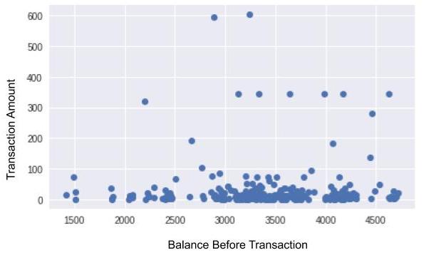
At first glance, this dispersion diagram doesn’t appear to show that transaction amounts are particularly small when the balance is low. There doesn’t seem to be any correlation (although you may find one in your own statements!). However, there are many points and they are fairly spread out. It is therefore difficult to tell. To remedy this, there is a type of representation that may be better. You’ll find it in the Take It Further section at the end of this chapter!
Two Quantitative Variables: Numerical Indicators
Graphs are nice, but I sense that you are missing calculations! We need a numerical indicator that can tell us whether our variables are correlated.
Here, we want to know if, when we have a low balance (), we also have a small transaction amount (). But small in relation to what? Here, when we say “small,” we mean in relation to other values, so what we’re saying is: “below the mean.” Let’s take a random banking transaction (= an individual), and use to refer to the balance before a transaction, and to refer to the amount of the transaction. To measure whether is below the mean, we can calculate as follows:
If x is below , this amount will be negative; if it is above , it will be positive. Similarly, to compare y to the mean , we can calculate . Now, let’s multiply them!
\(a=(x - \overline{x})(y-\overline{y})\)
If \(x\) is below the mean, and \(y\) is below the mean, both will be negative. When we multiply two negative numbers, we obtain a positive number. This also works in the other direction: if \(x\) is above the mean and \(y\) is above the mean, then \(a\)will be positive number.
So with this multiplication, we obtain the amount for a single banking transaction (a single individual). But if the amounts are truly small when the balance is low (and vice-versa), the s of all of the transactions will be positive! And if we find the mean of all of these s, we will still get a positive number. The mean of all of these as is written as follows:
To conclude: if is low when is small (and vice-versa), then will be positive. If, on the other hand, and are not correlated, will instead be close to 0. The more motivated among us will also deduce that if is high when is small (and vice-versa), then will be negative. In this case, there is a correlation, of course, but it is referred to as a negative correlation.
The Empirical Covariance and the Correlation Coefficient
Guess what! The indicator we just developed is commonly used in statistics; it’s called the Empirical Covariance of X and Y. Does this term remind you of the Empirical Variance? It should: they are similar. That’s right, if you calculate the empirical covariance of X and Y, you will find yourself using the formula for the empirical variance of X, which is written .
Magic!
To bring the empirical covariance to a value of between -1 and 1, we can divide it by the product of the standard deviations. This normalization enables us to make comparisons. This gives us:
This r coefficient is referred to as the correlation coefficient, the linear correlation coefficient, or sometimes Pearson’s correlation coefficient.
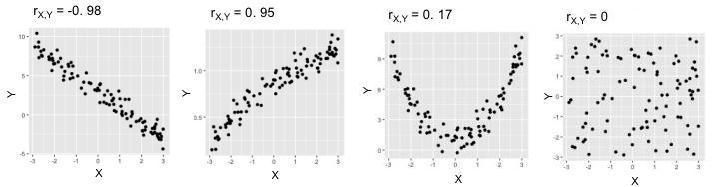
Why "Linear"?
Because, unfortunately, it only detects relationships when they are linear, that is, when the points line up more or less in a straight line. In the plots below, the two on the left show points in fairly straight lines: their s are therefore close to 1 or -1. In the fourth plot, however, there is no real correlation (knowing the value of a point gives us no indication as to its value) and therefore is close to 0. In the third plot, there is a strong correlation, but its shape is not linear; therefore is also unfortunately close to 0.
Now for the code…
Here is the code for generating the scatter plot seen at the beginning of this chapter:
import matplotlib.pyplot as plt

expenses = data[data.amount < 0]
plt.plot(expenses["balance_bef_trn"],-expenses["amount"],'o',alpha=0.5)
plt.xlabel("balance before transaction")
plt.ylabel("expense amount")
plt.show()
Now, to calculate Pearson’s coefficient and the covariance, you need only two lines!
import scipy.stats as st
import numpy as np

st.pearsonr(expenses["balance_bef_trn"],-expenses["amount"])[0]
np.cov(expenses["balance_bef_trn"],-expenses["amount"],ddof=0)[1,0]
The linear correlation coefficient is calculated by calling the st.pearsonr method. We then give it the two variables to be analyzed. Note that, in this chapter, we prefer to make our expense amounts positive, which is why there is a minus sign - before expenses["amount"] . A pair of values is returned. The first member of this pair is the correlation coefficient, which is why there is a[0] at the end of line 4.
The np.cov method returns the covariance matrix, which you don’t need to know about at this level. This matrix is in fact a table, and in this table, it is the value in the second row of the first column, which is why the code contains [1,0] .
Take It Further: Alternative to Dispersion Diagrams
To obtain a clearer representation than a scatter plot, we can aggregate the X variable into interval bins along the horizontal axis. This is equivalent to “cutting” the previous graph into vertical slices. For each slice, we display a box plot calculated from all of the points in the slice. Here is the new graph we obtain:
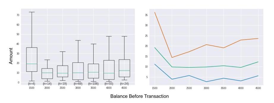 In the graph on the left, we can’t really tell whether the lower balance is, the smaller the amount will be, even though the box plots for slices [2000;2500[ and [2500;3000[ seem slightly denser at the top. The box plot furthest to the left is very dispersed; this may seem surprising, but in fact it is not very representative, because it represents only 4 individuals out of a population of almost 300. Note, therefore, that it is important to display the occurrences for each bin (n=4, n=14, n=19, etc.).
bin_size = 500 # size of bins for discretization

groups = [] # will receive the aggregated data to be displayed

# slices are calculated from 0 to the maximum balance in increments of bin_size]
slices = np.arange(0, max(expenses["balance_bef_trn"]), bin_size)
slices += bin_size/2 # slices are separated by half a bin size
indices = np.digitize(expenses["balance_bef_trn"], slices) # associates each balance with its bin number

for ind, tr in enumerate(slices): # for each slice, ind receives the slice number and tr the slice in question
    amounts = -expenses.loc[indices==ind,"amount"] # selects individuals for the ind slice
    if len(amounts) > 0:
        g = {
            'values': amounts,
            'bin_center': tr-(bin_size/2),
            'size': len(amounts),
            'quartiles': [np.percentile(amounts,p) for p in [25,50,75]]
        }
        groups.append(g)
# display box plots

plt.boxplot([g["values"] for g in groups],
            positions= [g["bin_center"] for g in groups], # X-axis of box plots
            showfliers= False, # outliers are not included
            widths= bin_size*0.7, # graph width of box plots
           )
# displays occurrences for each bin

for g in groups:
    plt.text(g["bin_center"],0,"(n={})".format(g["size"]),horizontalalignment='center',verticalalignment='top')
plt.show()
# display quartiles

for n_quartile in range(3):
    plt.plot([g["bin_center"] for g in groups],
             [g["quartiles"][n_quartile] for g in groups])
plt.show()
Take It Further: Properties of the Empirical Covariance
Very briefly, here are two properties of the Empirical Covariance:
. This is the property of symmetry.
If we create a new variable from two variables and V whose empirical covariance is known, and , then . This is the property of bilinearity.
