Analyze Two Quantitative Variables using Linear Regression
In the last chapter, we studied the correlation between two quantitative variables. Let’s continue now with two other variables, also quantitative: wait and amount.
The wait variable is populated only for banking transactions in the GROCERIES category. In a previous chapter, you perhaps added values to the GROCERIES category for some of your banking transactions. If this is not the case, I invite you to go back now and download the enriched_operations.csv sample.
A transaction’s wait variable gives the number of days that have elapsed between the current and previous transaction in the GROCERIES category. If you buy groceries every seven days on average, the mean of wait will be 7.
What do we expect to find?
In theory, the longer you wait to buy groceries, the more you will need to buy. So we expect that the higher the wait value is, the larger the amount value will be.
The Preliminary Step
First, we need to calculate the wait variable! Here is the code (you don’t necessarily need to understand it):
import datetime as dt

# Sub-sample is selected
groceries = data[data.categ == "GROCERIES"]

# Transactions are sorted by date
groceries = groceries.sort_values("transaction_date")

# Expenses are converted to positive amounts
groceries["amount"] = -groceries["amount"]

# Wait variable is calculated
r = []
last_date = dt.datetime.now()
for i,row in groceries.iterrows():
    days = (row["transaction_date"]-last_date).days
    if days == 0:
        r.append(r[-1])
    else:
        r.append(days)
    last_date = row["transaction_date"]
groceries["wait"] = r
groceries = groceries.iloc[1:,]

# transactions made on the same date are grouped together
# (groceries bought the same day but in 2 different stores)
a = groceries.groupby("transaction_date")["amount"].sum()
b = groceries.groupby("transaction_date")["wait"].first()
groceries = pd.DataFrame([a for a in zip(a,b)])
groceries.columns = ["amount","wait"]
Here we create a sub-sample that contains only tra nsactions in the groceries category, and call it... groceries!
Let’s Model It!
But we are going to do better than that: we are going to calculate the average cost for the products you consume in one day, and the speed at which you stockpile products in your pantry! To do this, we will use a model. You’ll see: it’s very powerful.
For the model we’re creating, we are going to make a number of assumptions. First, we will assume that each time you buy groceries, you buy three types of products:
Products you will consume before you buy groceries again (food, hygiene products, etc.).
Products you will not consume during the period being analyzed (this being the time between the first and last receipts you recorded in the sample): this is your long-term stockpile (jars of jam, frozen foods, etc.).
Products that are not consumable (ex: forks, floor cloths, etc.), which you buy only rarely.
Next, we will assume that you consume products every day, and that the cost of the products you consume in one day is more or less consistent.
Let’s refer to the average cost of the products you consume in one day (type 1) as a, and to the average cost of the products you don’t consume (type 2 and 3 together, which we assume you buy every time you go shopping) as . Finally, let’s refer to the number of days you waited since the last time you bought groceries as \(x\)$, and to the amount of the receipt as \(y\)$.
What will the amount of your next grocery receipt be?
It will be equal to the number of days you waited, multiplied by the average cost of what you consume in one day. But we also need to factor in the average cost of type 2 and 3 products. This gives the following formula:
Yes, our model is simplistic! The equation is not exact. You will also have noticed, no doubt, that it’s a linear equation (remember our affine functions). The fact that it’s a linear equation means that if I take all of the possible s between, for example, 0 and 5, and calculate all of their associated s before placing them on a graph with the s on the horizontal axis and les s on the vertical axis, all of the points will line up perfectly! So let’s try to display a scatter plot where X = wait and Y = amount, and see if all of the points line up:
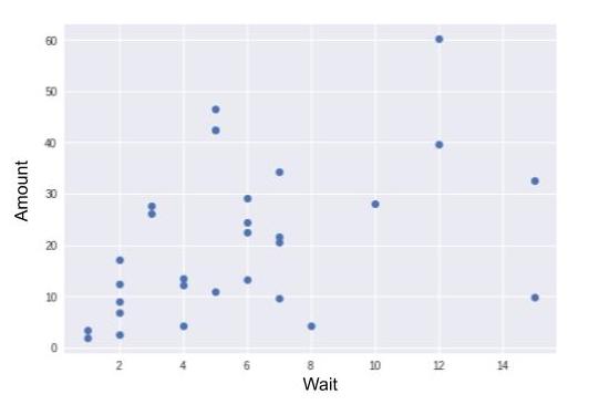
Far from it! This means that the equation is not perfectly accurate: it’s simplistic. With this equation, I admit that there will be an error between my predicted value and the actual value of the next receipt. But I can incorporate this error into the equation, calling it (epsilon):
To calculate and , I could simply take values at random. But if I did, the error ϵ would often be quite large. What I want is to keep my error as small as possible. I am looking to minimize the error.
This is how we could represent things graphically. By varying and , I shift the line on the graph. Minimizing the error means placing the line in general alignment with the points. The following illustration is for the purposes of instruction; almost all of the points fall into a straight line:
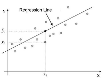
We see that for a point , we want the difference between (which is the true value) and (which is the value predicted by my inexact equation of ) to be minimal.
The computer can estimate and for us. To find out more, go to the Take It Further section. The following estimates are obtained:
At the beginning of this chapter, we made some assumptions. Simply put, we assumed that there was a linear connection between wait and amount; that is, a type connection. But is this assumption realistic? After applying a model, you must always analyze its quality. I therefore urge you to read the section Take It Further: Analyzing Model Quality.
Let’s Critique the Result!
The results indicate that the cost of what I consume daily is only $1.74. That doesn’t seem like much! In addition, $10.94 for long-term supplies every time I buy groceries? That’s huge!
So, it’s true ... looking at it more closely, I see that two points have “broken away from the pack.” We call these outliers. Being familiar with my own consumer habits, I know that I never wait more than 15 days to buy groceries. These two outlier points, for which the wait value = 15 days, correspond, in fact, to times when I had just returned from vacation (during which I did not buy groceries). Since I don’t want these outliers to interfere with my calculation, I discard them.
Once these have been discarded, I obtain the following new estimates:
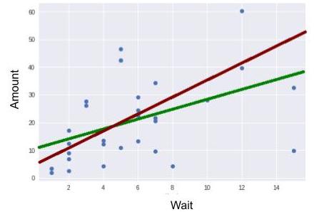
This result is quite different from the previous one. Discarding just two individuals significantly altered the outcome. We can therefore conclude that the statistical model we just applied (linear regression estimates using the method of least squares) is very sensitive to outliers.
Take It Further: Analyzing Model Quality
Imagine that I accidentally deleted the amount of a banking transaction in the GROCERIES category.
I could fill in this missing value with the mean of my transaction amounts. This is the most basic solution there is, and as you can imagine, it’s not very good! It’s not very good because amount values vary around the mean, sometimes by a lot.
I can do better: I can look at the value of the wait variable for this transaction. Using the linear regression model I developed, I can estimate the value (using the equation ). As I’m sure you’ve guessed, this estimate will be better than the one before. That’s right: when we were trying to minimize the modeling error, we were in fact trying to minimize variations in amount values around the regression line.
If we had found a perfect model, there would be no error, and no more variations between predicted and actual values. In this case, we would say that the model explained all of the variations. Variations around the mean are measured in terms of variance. A perfect model would explain 100% of the variations.
This percentage is calculated using the analysis of variance formula (ANOVA).
TSS (Total Sum of Squares) translates the total variation of Y. ESS (Explained Sum of Squares) translates the variation explained by the model. And RSS (Residual Sum of Squares) translates the variation that is not explained by the model.
For linear regression, the explained percentage of variation is given by the coefficient of determination, which is written:
Take It Further: Estimating and
Here are the formulas used to estimate and :
Why are there circumflexes over the and the ?
This is an estimating convention. It is thought that you can’t directly access your consumer behavior, characterized by and , but that you can estimate your behavior using your receipts. Estimates of and are therefore written and ̂ .
If we added a new receipt to the sample, and ̂ would vary somewhat, even if your consumer behavior didn’t change (that is, even if and “didn’t move”).
How do we estimate and in the code?
See below. The code here is a little complicated, but remember that line 6 creates the variables a and b that contain the estimates.
import statsmodels.api as sm

Y = groceries['amount']
X = groceries[['wait']]
X = X.copy() # X will be modified, so a copy is created
X['intercept'] = 1.
result = sm.OLS(Y, X).fit() # OLS = Ordinary Least Squares
a,b = result.params['wait'],result.params['intercept']
To display the line, proceed as follows:
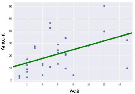
plt.plot(groceries.wait,groceries.amount, "o")
plt.plot(np.arange(15),[a*x+b for x in np.arange(15)])
plt.xlabel("wait")
plt.ylabel("amount")
plt.show()
Line 1 displays the scatter plot.
On line 2, np.arange creates a list of whole numbers from 0 to 14: [0,1,2,3,4,5,6,7,8,9,10,11,12,13,14] .
We place this list on the X-axis. We calculate the ordinates for each of these 15 values using the formula y=ax+b: [a*x+b for x in np.arange(15)] . In so doing, we create a series of points, all of which line up around the straight line of the equation y=ax+b. Line 2 displays all of these points, arranging them in a nice little line!
