Perform an Initial Data Analysis

Okay... all that’s left now is to analyze two qualitative variables. Let me to reassure you: you did half the work already in the chapter on contingency tables. If you understood that principle, you’re well ahead of the game.

Questions We Can Ask

The method of analysis will be the same no matter which of the following questions you ask. The only thing that changes is the variable pair:

• Do I have the same expense categories on the weekend as during the week? (categ and weekend)

• Do I have more money coming in at the beginning of the month or at the end of the month? (debcr and quart_month)

• Are my expense amounts larger at the beginning of the month than at the end of the month? (expense_slice and quart_month)

• Do my transaction amounts vary from one expense category to the next? (expense_slice and categ)

• Are my charge payments always small and my deposits always large? (type and expense_slice)

• Are there transaction categories that occur always at the same time of the month, such as rent, for example? (categ and quart_month)

• Are there transaction categories for which the form of payment is always the same, for example bank transfer? (type and categ)

 Representation

To answer these questions, you can display a contingency table as follows:

X = "quart_month"
Y = "categ"

cont = data[[X,Y]].pivot_table(index=X,columns=Y,aggfunc=len,margins=True,margins_name="Total")
cont

Replace the two qualitative variables on lines 1 and 2 with those you wish to analyze. The contingency table is calculated using the   pivot_table  method. Each cell in the contingency table counts a number of individuals. This count is performed using the  len function. 

 Use Statistics

Unfortunately, we won’t be able to use a model like we did in the last two chapters. But don’t worry! We’ll put things right using a statistical measurement.

Let’s go back to the chapter on contingency tables and look again at what we wrote in the sidebar:

If two events  $\$\backslash (I\backslash )\$$ and  $\$\backslash (J\backslash )\$$  are independent of one another, we expect the number of individuals that satisfy both  $\$\backslash (I\backslash )\$$ and $\$\backslash (J\backslash )\$$ (let’s call that number  $\$\backslash (n\_\{ij\}\backslash )\$$  ) to be equal to  $\$\backslash (f\_i\backslash times\; n\_j\backslash )\$$ (this is the calculation you made at the outset: 30% x 10 = 3). On the other hand, the more  $\$\backslash (n\_\{ij\}\backslash )\$$ differs from  $\$\backslash (f\_i\backslash times\; n\_j\backslash )\$$ , the more reason we have to believe that  $\$\backslash (I\backslash )\$$  and  $\$\backslash (J\backslash )\$$  are not independent.

So, analyzing the correlation between two qualitative variables is the same as comparing the  $\$\backslash (n\_\{ij\}\backslash )\$$ s to the  $\$\backslash (f\_i\backslash times\; n\_j\backslash )\$$s. The  $\$\backslash (n\_\{ij\}\backslash )\$$ s are numbers in the contingency table (except for the TOTAL rows and columns). We could therefore create another table in the same form as the contingency table, but containing the  $\$\backslash (f\_i\backslash times\; n\_j\backslash )\$$s instead. Here, then, on the left, is the contingency table that we had before and, on the right, the  $\$\backslash (f\_i\backslash times\; n\_j\backslash )\$$ table:

Table 2 is what we would expect if the two variables were independent. So we need a statistic that compares the values of these two tables, and that enables us to pinpoint the pairs of cells whose values really differ. These cells will contain values worthy of interest, and will be the source of non-independence between the two variables.

Here we go! If you want to compare two numbers, I suggest you calculate their difference! And to make sure our differences are always positive (to avoid canceling them out by adding them together), let’s square them. This is not the first time we’ve used this little stratagem:

$\$\backslash ((n\_\{ij\}\; -\; f\_\{i\}.n\_j)^2\backslash )\$$

 That’s true. So we can normalize this difference when squared by dividing it by $\$\backslash (f\_i.n\_j\backslash )\$$. We then obtain the following formula, knowing that  $\$\backslash (f\_i\; =\; \backslash frac\{n\_i\}\{n\}\backslash )\$$ :  

 $\$\backslash (\backslash xi\_\{ij\}=\backslash frac\{(n\_\{ij\}-\backslash frac\{n\_i.n\_j\}\{n\})^2\}\{\backslash frac\{n\_i.n\_j\}\{n\}\}\backslash )\$$ 

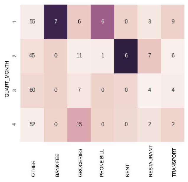
This measure can be calculated for each cell of the contingency table. It might be interesting to color-code the table according to the results, using dark colors for large results, and light ones for results of close to 0. That way, we can easily tell which cells are the source of non-independence:

 Finally, if we add up all of these  $\$\backslash (\backslash xi\_\{ij\}\backslash )\$$  measures for each cell of the table (from column j=1 to column j=I, and from row i=1 to row i=k), we obtain the statistic  $\$\backslash (\backslash xi\_n\backslash )\$$  ($\$\backslash (\backslash xi\backslash )\$$  is pronounced “zai” or “sigh”): 

 $\$\backslash (\backslash xi\_n\; =\; \backslash sum\_\{i=1\}^k\backslash sum\_\{j=1\}^l\backslash frac\{(n\_\{ij\}-\backslash frac\{n\_i.n\_j\}\{n\})^2\}\{\backslash frac\{n\_i.n\_j\}\{n\}\}\backslash )\$$

Normally, we apply a threshold to this measure, above which we say that the two variables are correlated. It’s a little complicated, but here, we simply need to remember that the larger  $\$\backslash (\$\backslash )\$$\(\xi_n\)$is, the less likely it is that any hypothesis of independence will be valid.

As we have seen, we can associate each cell of the table with a $\$\backslash (\backslash xi\_\{ij\}\backslash )\$$. We can then normalize each $\$\backslash (\backslash xi\_\{ij\}\backslash )\$$   by dividing it by  $\$\backslash (\backslash xi\_n\backslash )\$$. We then obtain for each cell a value of between 0 and 1.

This value can be considered a contribution to non-independence. Optionally, it can be expressed as a percentage, by multiplying it by 100. The closer this contribution gets to 100%, the more the cell in question will be considered a source of non-independence. The sum of all of the contributions is equal to 100%.

Here is the code for generating the color-coded contingency table:

tx = pd.DataFrame(tx)

ty = pd.DataFrame(ty)
tx.columns = ["foo"]
ty.columns = ["foo"]
n = len(data)
indep = tx.dot(ty.T) / n

c = c.fillna(0) # Null values are replaced by 0
measure = (c-indep)**2/indep
xi_n = measure.sum().sum()
sns.heatmap(measure/xi_n,annot=c)
plt.show()

 
Lines 1 to 6 calculate the   indep   table, which is the table representing independence. It calls the matrix product (.dot()), which you don’t need to know about at this level.

On line 9,  measure  contains all of the  $\$\backslash (\backslash xi\_\{ij\}\backslash )\$$  for each cell of the table. We can then calculate the contributions (defined above), dividing each $\$\backslash (\backslash xi\_\{ij\}\backslash )\$$ by $\$\backslash (\backslash xi\_n\backslash )\$$  (placed within the variable  xi_n ). We do this on line 11 with   measure/xi_n. We then obtain a value of between 0 and 1 for each cell.