Analyze One Quantitative and One Qualitative Variable using ANOVA
In the last two chapters, we studied correlations between two quantitative variables. Now we’ll move on to two more variables, one of which is qualitative, the other quantitative.
Questions We Can Ask
Depending on which variable pair we choose, the method of analysis will be the same, but there are many different questions we can ask:
Are the purchases I make on weekends larger than the purchases I make during the week? (variables amount and weekend)
Are my purchase amounts larger at the beginning of the month than at the end of the month? (amount and quart_month)
Do my transaction amounts vary from one expense category to the next? (amount and categ)
Are my charge payments always small and my deposits always large? (type and amount)
Is the balance in my account lower at the end of the month than at the beginning of the month? (balance_bef_transaction and quart_month)
Graphs!
Here is the code for representing a quantitative variable and a qualitative variable. First, create your working sub-sample, adapting the code, in particular the X and Y variables, to the question you selected from the list above.
X = "categ" # qualitative
Y = "amount" # quantitative

# Only expenses are retained
sub_sample = data[data["amount"] < 0].copy()
# Expenses are converted to positive amounts
sub_sample["amount"] = -sub_sample["amount"]
# Rents are not included because too large:
sub_sample = sub_sample[sub_sample["categ"] != "RENT"]
After which, these six lines of code will display your graph!
categories = sub_sample[X].unique()
groups = []
for m in categories:
    groups.append(sub_sample[sub_sample[X]==m][Y])

# Graph properties (not very important)
medianprops = {'color':"black"}
meanprops = {'marker':'o', 'markeredgecolor':'black',
            'markerfacecolor':'firebrick'}

plt.boxplot(groups, labels=categories, showfliers=False, medianprops=medianprops,
            vert=False, patch_artist=True, showmeans=True, meanprops=meanprops)
plt.show()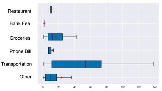
Here we see that the amounts vary greatly from one category to the next. For example, transportation expense amounts are higher and more broadly dispersed than phone bill expense amounts. But now let’s verify this with figures, using a model.
Model the Data
Let’s revisit the approach we took in the last chapter. To find out whether there was a (linear) correlation between two variables, we assumed that this correlation existed, then applied a model to this assumption. Next we estimated the and parameters. Finally, we verified the initial assumption by evaluating the quality of our model. If our model is high quality, there will be a strong correlation between X and Y. As a bonus, we took advantage of the linear regression formula to interpret as the cost of what we consume in one day, and as the cost of our stockpile and non consumable products.
We will take the same approach here.
We could use the same linear regression formula as above, but it requires multiplying by and, this time, X is qualitative, like our categ variable. Multiplying a qualitative variable by a number is not meaningful (ex: “TRANSPORT” x 3 makes no sense!).
So we’re going to take another approach. We will assume that our banking transactions have a common reference amount . We will then assume that the transaction amount varies according to the expense category (rent, transportation, groceries, etc.). If a category contains amounts that are generally lower than , the adjustment will be negative. If the opposite is true, the adjustment will be positive. We add the requirement that the sum of all of the s be equal to 0.
Just like in the previous chapter, your prediction will always be erroneous, because the amounts are not all the same within the same category!
This is true. And, just as we did with our linear regression model, we will use an error term:
\(Y = \alpha_{i} + \mu + \epsilon\)$
As in the previous chapter, the computer can estimate all of the s and s, except here, the mathematical calculations that tell us which and minimize the error give very intuitive results:
The reference amount is estimated using the mean of all of the amounts. We call this estimate .
For a category , is estimated by calculating the difference between and the mean of the amounts in the category , that is,
Evaluating the Model: Are the Variables Correlated?
Is ours a good quality model? Are we correctly predicting transaction amounts based only on their category?
As in the previous chapter, we hope that our model is able to explain a high percentage of variations in the data. If it does, it means that there is a strong correlation between our categ and amount variables .
To evaluate our model, we use exactly the same formula as in the previous chapter: . But here, because variable X is qualitative, we can use expressions for TSS, ESS and RSS that are equivalent to those in the previous chapter. They are provided in the Take It Further section. These expressions also allow for better interpretation of the three acronyms, which can be renamed, respectively, total variation, inter-classvariation, and intra-classvariation (the classes being the categories of our X variable).
In the last chapter we had . Here we have the equivalent: the correlation ratio, between 0 and 1, given by:
If , the means per category are all equal. There is therefore theoretically no relationship between variables Y and X. However, if , the means per category are very different, each of the categories being made up of identical values: there is therefore theoretically a relationship between variables Y and X.
Here is the code for calculating (eta squared). I suggest you perform this calculation by hand: ;)
X = "categ" # qualitative
Y = "amount" # quantitative

sub_sample = data[data["amount"] < 0] # Only expenses are retained

def eta_squared(x,y):
    mean_y = y.mean()
    categories = []
    for category in x.unique():
        yi_category = y[x==category]
        categories.append({'ni': len(yi_category),
                        'mean_category': yi_category.mean()})
    TSS = sum([(yj-mean_y)**2 for yj in y])
    ESS = sum([c['ni']*(c['mean_category']-mean_y)**2 for c in categories])
    return ESS/TSS

eta_squared(sub_sample[X],sub_sample[Y])
We obtain a result of close to 0.4, which leads us to believe that there is definitely a correlation between the expense amount and the category. Which is what we observed in the graph at the beginning of the chapter!
Take It Further: TSS, ESS and RSS Expressions
TSS, ESS and RSS expressions introduce the occurrences of each of the categories , which are in number. So:
