Design Effective Statistical Models to Understand Your Data

There are two main approaches in statistical modeling: exploratory and predictive.

In the exploratory approach, our goal is to understand the relationships between predictors X and a target variable y. We want to answer the question: when X increases by a unit, by how much can we expect y to increase or decrease?

In the predictive approach, we want to build a model that is able to predict the target variable for previously unseen values of the predictors.

• Using a simple example of Weight vs. Height in schoolchildren, we want to estimate the weight for really tall children not in the dataset.

• In the auto-mpg dataset, we want to see how the miles per gallon variable increases for very heavy cars also not included in the dataset

• In the Ozone dataset, we want to extrapolate the effect of an increase in temperature on the level of ozone.

To build models that can make reliable predictions on new data, you need to be able to measure the quality of these predictions. This entails a new way of measuring the performance of the model and techniques on how to exploit a dataset to simulate the model's behavior on new data.

In this chapter, you will learn the following:

• How to measure the performance of a linear regression model using RMSE.

• How to split your dataset into a training and testing subsets to score your model.

• The impact of outliers.

• How to detect overfitting.

• How to select the most robust model with regards to outliers using k-fold cross-validation.

Let's get to work!

Evaluating the Predictive Performance of a Regression Model

As you've seen in previous chapters, you have a wide range of statistical tests at your disposal as well as their associated p-values, statistics and confidence intervals to assess the quality of a model and select the best among several competing ones. But you don't have a measure of how close or how far your model is from the real values of the outcome variable.

The Root Mean Square Error

When you model a target variable $\$\backslash (y\backslash )\$$ , you want to know the distance between $\$\backslash (y\backslash )\$$ and the output of your model $\$\backslash (\backslash hat\{y\}\backslash )\$$. For that, you use the metric called RMSE or Root Mean Square Error, which is defined as:

$\$\backslash [RMSE\; =\; \backslash sqrt\{\; \backslash frac\{1\}\{n\}\; \backslash sum\_\{i=1\}^n\; (\backslash hat\{y\}\_i\; -\; y\_i)^2\; \}\backslash ]\$$

The RMSE is the square root of the  sum of the square of all the residuals divided by the number of samples (N). The RMSE is a relative number which increases with the average of $\$\backslash (y\backslash )\$$ and $\$\backslash (\backslash hat\{y\}\backslash )\$$ .

In Practice

Let's put that to practice and compare several models built on the Ozone dataset. We'll define and fit six different models, calculate their RMSE on the whole dataset, and see which one has the lowest RMSE. Here are the models:

• M1: Ozone ~ Temp

• M2: Ozone ~ Temp + Temp^2

• M3: Ozone ~ Wind

• M4: Ozone ~ Wind + Wind^2

• M5: Ozone ~ Temp + Wind + Solar

• M6: Ozone ~ Temp + Temp^2 + Wind + Wind ^2 + Solar

Let's load the data, remove the missing values, rename a column, and create Wind^2 and Temp^2 columns:

df = pd.read_csv('ozone.csv')
df = df.dropna().rename(columns = {'Solar.R': 'Solar'})
df['Wind2'] = np.square(df['Wind'])
df['Temp2'] = np.square(df['Temp'])

Let's now define a function that calculates the RMSE given the residuals of the model:

def RMSE(resid):
    return np.sqrt(np.square(resid).sum()) / len(resid)

Since we have many models to test, it's best to loop through them, and for each one, record the RMSE. For that, we'll define an array with the different formulas of the models:

formulas = ['Ozone ~ Temp',
'Ozone ~ Temp + Temp2',
'Ozone ~ Wind',
'Ozone ~ Wind + Wind2',
'Ozone ~ Temp + Wind + Solar',
'Ozone ~ Temp + Temp2 + Wind + Wind2 + Solar'
]

Now we can loop through each formula, creating and fitting each associated model:

scores = []
for formula in formulas:
    results = smf.ols(formula, df).fit()
    scores.append( { 'model': formula,
        'RMSE':RMSE(results.resid),
        'R-squared': results.rsquared} 
    )

scores = pd.DataFrame(scores)

In this script, fit each model, calculate the RMSE based on the residuals of the model, and stack the scores in the scores list.

In the end you have:

print(scores.sort_values(by = 'RMSE').reset_index(drop = True))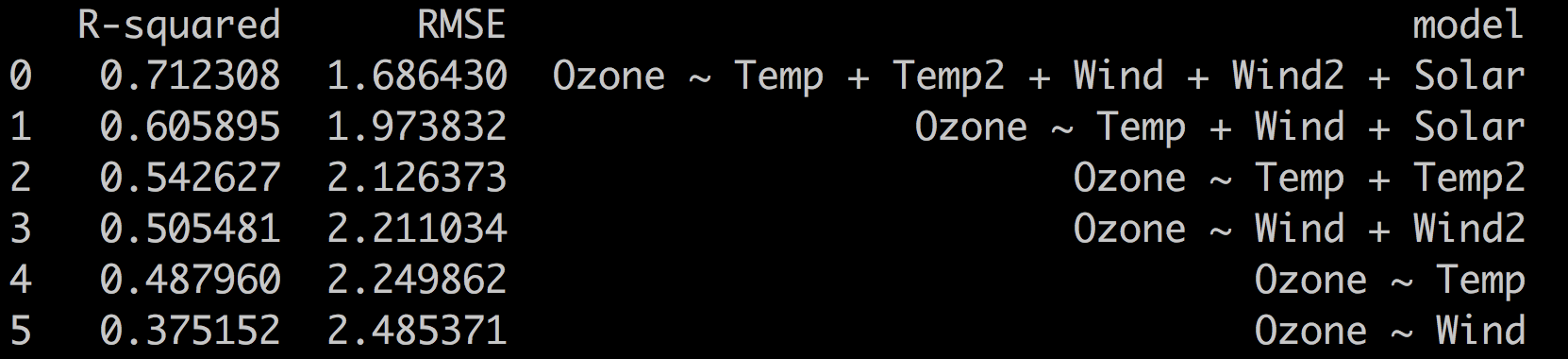

The RMSE aligns with the R-squared metric. The best model is the most complex one
 $\$\backslash (M6:\; Ozone\; \backslash sim\; Temp\; +\; Temp^2\; +\; Wind\; +\; Wind^2\; +\; Solar\backslash )\$$ with the lowest RMSE and highest R-squared.

At this stage, if you were trying to understand the relationships between the variables, it would make sense to look at the p-values, t-statistic, and confidence intervals for each of the coefficients of the regression. As you've seen in the previous chapters, adding variables to the model can have side effects (multicollinearity, for instance) that render the regression coefficients non-reliable.

Right now, we're only interested in how the model reflects the existing data. And since we're building a model for prediction, the main concern will be with overfitting. Is the model too complex for its own good? Is it too dependent and sensitive on the dataset?

Overfitting

So far we've used all the samples in our dataset to estimate of the coefficients of the regression through the OLS method. In other terms, we've used our entire dataset to train our model.

In general, there are two steps when training a model.

The model definition part:

model = msf.ols(formula, data = df)

The model fitting part:

results = model.fit()

The fitting step is where you train the model to estimate the regression coefficients.

We have calculated the RMSE based on the whole dataset using the residuals of the model:  results.resid with  results.resid = df.Ozone - results.fittedvalues.

This RMSE score shows how good the model is at mimicking the target variable, but not how it will behave when dealing with previously unseen data. Will the predictions based on new values for temp, wind, and solar be reliable or off the charts?

In other words, is our model overfitting: good at mimicking the training dataset, but unable to generalize to new values.

Training and Testing Subsets

To measure how well the model performs on the training data as well as new unseen data, we are going to split our dataset into two subsets:

• A train subset on which we'll train (fit) the model.

• A test subset on which we'll calculate the RMSE.

Since the model has not seen the samples from the test subset during training, this score will give us a good indication of how the model behaves on unseen data.

To split the dataset randomly, sample  the index of the pandas DataFrame:

# take a random sample of 70% of the dataframe
train_index = df.sample(frac = 0.7).index
# create the train and test subset
train = df.loc[df.index.isin(train_index)]
test = df.loc[~df.index.isin(train_index)]

This gives 78 samples for our train set, and 33 for our test set.

Let's go over the six previous models, and this time, record the RMSE based on the test set.
For that, we will need to predict the values of the test set using  results.predict(test).

The code is very similar:

scores = []
for formula in formulas:
    results = smf.ols(formula, train).fit()
    yhat = results.predict(test)
    resid_test = yhat - test.Ozone
    scores.append( { 'model': formula,
        'RMSE_test':RMSE(resid_test),
        'RMSE_train':RMSE(results.resid),
        'R-squared': results.rsquared} 
    )

scores = pd.DataFrame(scores)

The only difference is in Lines 4 and 5 where we first make a prediction on the test  samples yhat = results.predict(test)  and calculate the residuals  resid_test = yhat - test.Ozone.

These are the results on the test set:

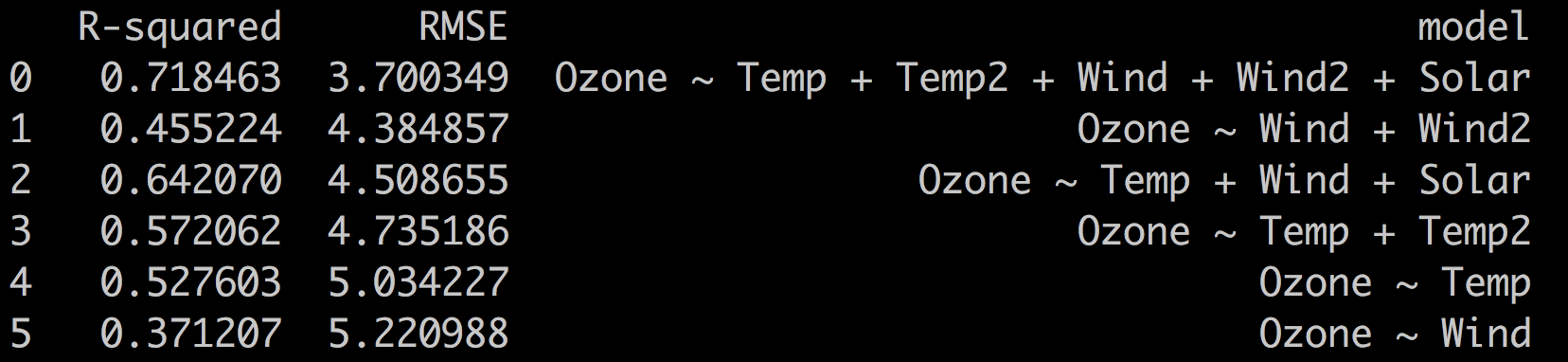
As you can see, the best model (the one with lowest RMSE) is still the most complex one: Ozone ~ Temp + Temp2 + Wind + Wind2 + Solar. But now, the Ozone ~ Wind + Wind2 performs better than Ozone ~ Temp + Wind + Solar, which was not the case in our previous iteration.

Notice that the values of RMSE have changed since the data on which it was calculated has also changed. What's important here is the relative value of the RMSE.

Overfitting Anyone?

Here's how it works. Let's say you are comparing different models that are more and more complex. In the context of linear regression, this means that you're adding predictors to the linear model.

If you plot the RMSE_train and RMSE_test versus the increasing complexity of your models, you will get one of these two plots:

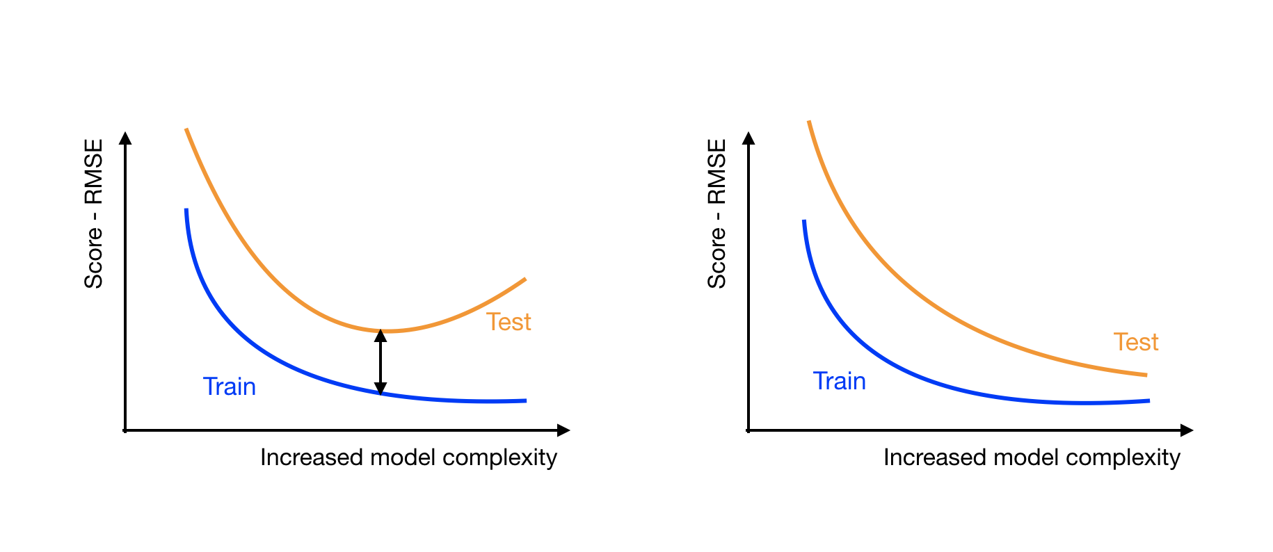
• On both plots, the RMSE train (blue) decreases with the complexity of the model. This means that the more complex models are better at fitting the training data.

• On the left plot, the RMSE test score (orange) decreases until it reaches a minimum, and then starts increasing.

• On the right plot, the test score keeps on getting lower and closer to the train RMSE.

The left plot shows that the more complex models are overfitting.  The point where the test score is the closest to the train score indicates the best model. When the test score starts increasing, the model starts to overfit the training data and is getting worse at handling unseen data.

The plot on the right shows that as you increase the complexity of the model, you're still gaining performance. At some point, the models may become too complex and start overfitting, but so far, so good. You should train and test more complex models to get lower test scores.

Hands On

Let's add extra complex models to our growing collection and see if some of them start overfitting. Some of them are a bit over the top. :soleil:

Create new predictors/features for each: solar, wind, and temp to the power of 4:

df['Wind3'] = df['Wind']**3
df['Wind4'] = df['Wind']**4
...
df['Temp4'] = df['Temp']**4

And define the following 11 models:

formulas = [
'Ozone ~ Solar',
'Ozone ~ Solar + Solar2',
'Ozone ~ Wind',
'Ozone ~ Wind + Wind2',
'Ozone ~ Temp',
'Ozone ~ Temp + Temp2',
'Ozone ~ Temp + Wind + Solar',
'Ozone ~ Temp + Temp2 + Wind + Wind2 + Solar + Solar2',
'Ozone ~ Temp + Temp2 + Temp3 + Wind + Wind2 + Wind3 + Solar + Solar2 + Solar3',
'Ozone ~ Temp + Temp2 + Temp3 + Temp4 + Wind + Wind2 + Wind3 + Wind4 + Solar + Solar2 + Solar3 + Solar4',
'Ozone ~ Temp + Temp2 + Temp3 + Temp4 + Wind + Wind2 + Wind3 + Wind4 + Solar + Solar2 + Solar3 + Solar4 + Temp * Wind + Temp * Solar + Wind * Solar',
]

Consider the original variable and its square, then the combinations of the three variables adding increasing powers to the set of predictors. In the last and most complex model, also add the cross variables to the mix:  Temp * Wind + Temp * Solar + Wind * Solar .

Plotting the RMSE_test and the RMSE_train you get:

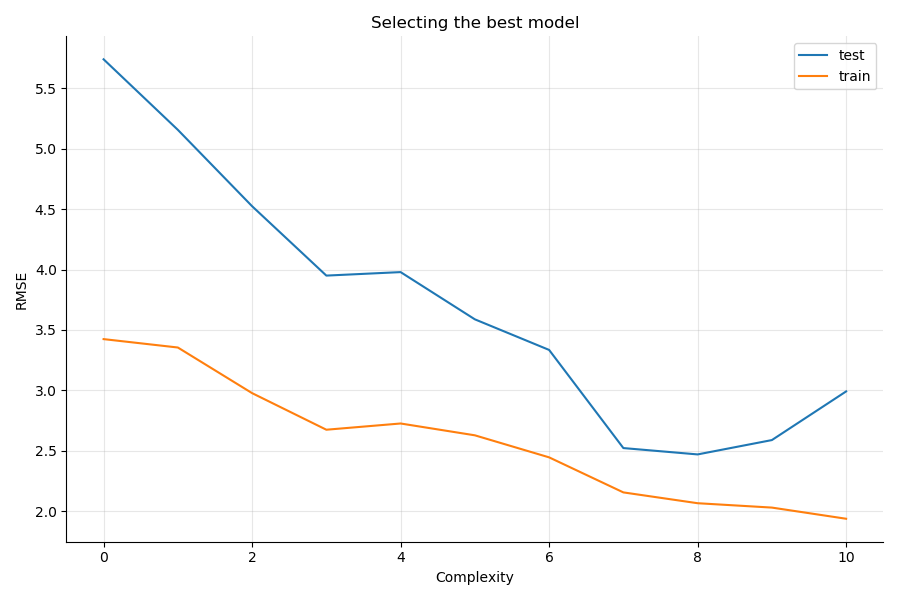
You see that the test RMSE decreases until model 7 and 8, and then increases again while the train RMSE keeps on decreasing as models have more and more predictors.

Model 6,7, and 8 correspond to:

'Ozone ~ Temp + Wind + Solar',
'Ozone ~ Temp + Temp2 + Wind + Wind2 + Solar + Solar2',
'Ozone ~ Temp + Temp2 + Temp3 + Wind + Wind2 + Wind3 + Solar + Solar2 + Solar3',

By adding the square of the original predictors, you gain significant performance; however,  adding the cube of the original predictors does not lead to any further significant RMSE reduction.

The best model in our situation is: Ozone ~ Temp + Temp2 + Wind + Wind2 + Solar + Solar2, as it offers the smallest gap between the train and test errors, and is simpler than the model involving the cubes of the original features.

K-Fold Cross-Validation

The Ozone dataset is quite small, with just over 110 samples, and the performance of the model may be very sensitive to the train/test dataset split. This is especially true if the dataset has some outliers or extreme data that end up only in the testing subset. The model won't be able to correctly handle extreme values it has not been trained on. Similarly, outliers only present in the training subset may have a significant impact on the model's coefficients, potentially leading to lower performances.

So if the performance of the model is dependent on how the data was split between train and test, there's a good chance you won't select the best model in the end.

To make sure you select the most robust model, run the train/test split multiple times and average the scores of all the runs. The model with the best score average is the most robust one and less prone to overfitting. This technique is called cross-validation.

There are multiple ways to implement cross-validation. We will focus on the most standard one: k-fold cross-validation.

To do k-fold cross-validation, split your dataset in k-subsets, use k-1 subsets to train the model, and use the remaining subset as the test set to score the model. The test subset is chosen in turn.

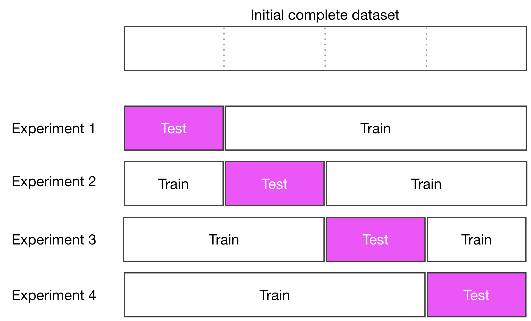
Implement K-Fold Cross-Validation

Implementing k-fold cross-validation is a matter of subsetting the dataset into k-subsets, and using the right subset for testing, and the others for training. For a given model,  run four experiments, each time training the model and evaluating its performances on a different chunk of the data. Now let's use that to compare our model using a 4-fold cross-validation.

The code goes like this:

K = 4
np.random.seed(8)
df = df.sample(frac = 1)
indexes = np.array_split(list(df.index),K)

scores = []

for formula in formulas:
    for i in range(K):
        test_index  = indexes[i]
        train_index = [idx for idx in list(df.index) if idx not in test_index]
        train = df.loc[df.index.isin(train_index)]
        test  = df.loc[~df.index.isin(train_index)]
    
        results = smf.ols(formula, train).fit()
        yhat    = results.predict(test)
        resid_test = yhat - test.Ozone
    
        scores.append( {
            'model': formula,
            'RMSE_test':RMSE(resid_test),
            'RMSE_train':RMSE(results.resid)
        })

scores = pd.DataFrame(scores)
scores = scores.groupby(by = 'model').mean().reset_index()

The new important things to focus on here are:

• l1: K is the number of folds you want to split the data into.

• l7: Loop over the list of formulas to define the model.

• l8: Iterate over the number of folds: K.

• l9 and l10:  These two lines are a rough way of getting successive test chunks from the data and complementary train indexes.

  test_index = indexes[i]
  train_index = [idx for idx in list(df.index) if idx not in test_index]

• l25: The last line is where you average the RMSE of the K different runs.

The rest of the code is similar to our previous implementation.

Obtain the following training/testing RMSE plot. Each point is the results of four different runs:

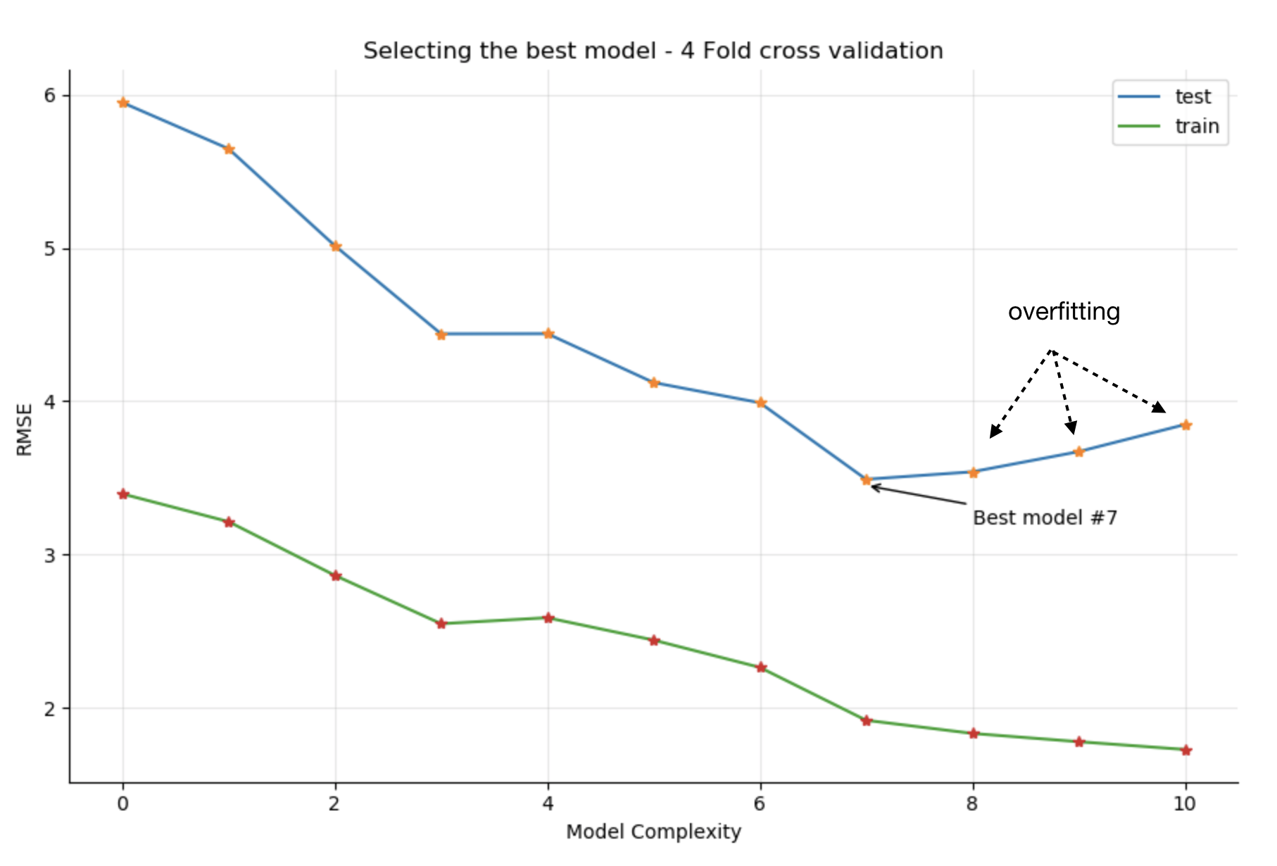
The best model is (again) #7  Ozone ~ Temp + Temp2 + Wind + Wind2 + Solar + Solar2 , and you now have confirmation that increasing the complexity of the model by considering the cube of the original predictors will only make the model overfit (models 8 and above) as the train RMSE decreases, but test RMSE starts increasing.

Although we end up selecting the same model as before (without cross-validation), we are more confident of the model's robustness and its predictive power.

Summary

In this chapter, we transitioned from pure statistical learning where the goal is to build models to explain and understand the dynamics at play within a dataset to machine learning, where the goal is to build predictive algorithms.

The key takeaways from this chapter are:

• The best model among equally performing models is always the simplest(Occam's razor).

• To evaluate the model performance on new data, split the dataset into a training and testing subset.

• Overfitting is when the model is too dependent on the training subset and unable to perform well on unseen data samples in the training subset.

• Overfitting can be detected by comparing the training score versus the testing score.

• K-fold cross-validation is a technique to reduce the sensitivity of the model score on the train/ test split.