Use Analysis Tools to Achieve Your Goals

Your boss is really happy with your dashboard! 😀
He has now asked you to work with him on a regional strategy, with the aim of achieving $150,000 of sales in Bulgaria in 2021. You are going to use analysis tools to help you.
Meet a Specific Target Using Goal Seek
Do you remember math lessons at school? Did you sometimes struggle to solve math problems?
Well, there’s no need to panic! This time, Excel is here to help! 😉
We need to start by setting out the problem.
What we know:
The average garment price is $8.20.
Packaging expenses are fixed at $623.
How many garments do we need to sell to achieve $150,000 in sales?
When entering this data into an Excel table, the calculation of the result is based on: result = number of sales x average garment price – fixed expenses.
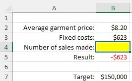
You’re going to use the Goal Seek feature to help Excel find the value of the yellow cell, which equates to the target number of sales.
Excel uses this tool to test out all possible values of a cell, to enable another cell to achieve a specific value.
In our example:
In the Data tab, click on “What-If Analysis”
 , then on the “Goal Seek” row.
In the “Set cell” field, select the cell which contains the result formula, i.e., B5.
Enter the value that you want to obtain, i.e., 150000.
In “By changing cell,” input the number of sales required (i.e., B4).
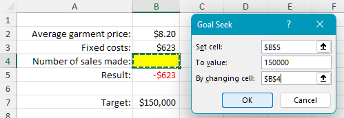
Click OK to prompt Excel to find the ideal value of B4, so that B5 can achieve its target value.
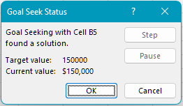
Click “OK” if you want to keep Excel’s value. Excel will populate cell B4. Otherwise, click Cancel.
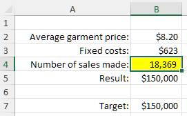
In this problem with just one unknown component, Excel has only taken a few seconds to find the solution! 😊
Solve Complex Problems Using Solver
If your problem includes more than one unknown, don’t panic! Solver is your friend!
What’s Solver?
Like Goal Seek, Solver is an analysis tool, but more in-depth. With Solver, your target can be:
an exact value (e.g., $50,000 sales target).
a minimum value (e.g., minimum $50,000 sales target).
a maximum value (e.g., what is the maximum number of sales that I can achieve with these criteria?).
What’s more, Solver lets you add limits (or “Constraints” as Excel calls them) to the problem, for example:
The production facility can only produce up to 1000 garments per month.
Raw materials for one garment cost between $5 and $10, depending on the supplier.
Excel can manage up to 200 cumulative constraints! 😀
Install the Solver Add-in
Excel does not install Solver by default. It is a free add-in which you simply activate.
To activate it:
Click on the “File” tab, then “Options” at the bottom of the screen.
Click the “Add-ins” menu, then “Go...” at the bottom of the screen.
The list of potential add-ins displays.
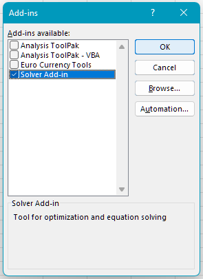
Check the box next to Solver Add-in, and click OK.
And there you have it! Solver is installed. 😊
Use Solver
Let’s go back to our problem. We want to achieve $150,000 of sales in Bulgaria in 2021.
You need to take into account the fact that the garments are priced differently in your sales projection. Moreover, you can only produce a certain number of garments per year, within the limits of your production facility.
Therefore:
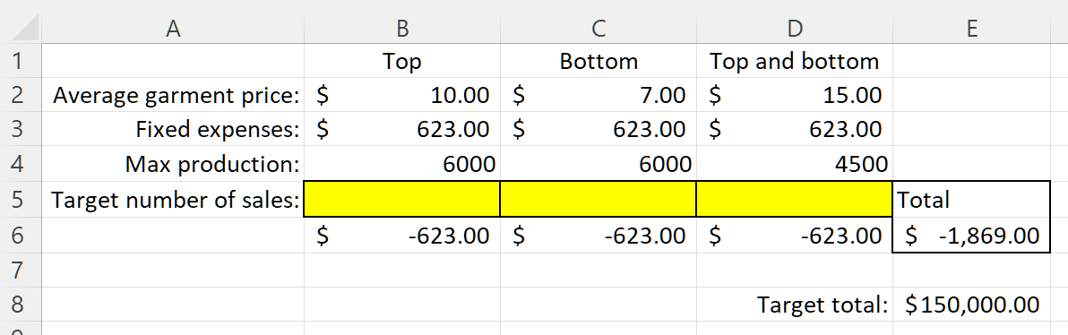
A garment in the “Top” category is priced at an average of $10, and its maximum production is 6000 units.
A garment in the “Bottom” category is priced at an average of $7, and its maximum production is 6000 units.
A garment in the “Top and Bottom” category is priced at an average of $15, and its maximum production is 4500 units.
The fixed packaging expenses for each clothing category are $623.
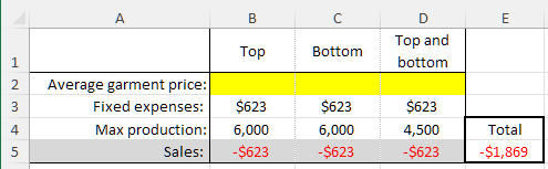
Incorporate all of this data into an Excel table, while keeping your target in mind.
Download this file to access the table.
You can solve this problem, which has multiples conditions, using Solver:
Go to the “Data” tab, “Analyze” group, and click the
 button.
The Solver window includes three fields:
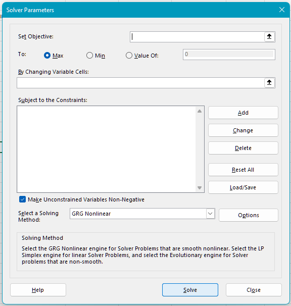
Set Objective, in this case, cell E6. And underneath, the value to be achieved: 150000.
The changing cells are the yellow cells (
B5:B5), which Solver will use to test out different combinations until it obtains the desired result.The Constraints, which are the limits of our problem:
Top sales should be 6000 units or under.
Bottom sales should be 6000 units or under.
Top and Bottom sales should be 4500 units or under.
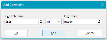
And you also need to tell Solver that values in the yellow cells must be whole numbers. After all, you can’t make 0.3 tops! 😊
In the Set Objective, select the cell which contains the calculation of the total, i.e., $E$6.
Check the “Value Of” box and add the value to be obtained, in this case, 150000.
Click “Add” to set up the first constraint, which will tell Excel that Top sales (cell B5) should not exceed 6000 units (cell B4).
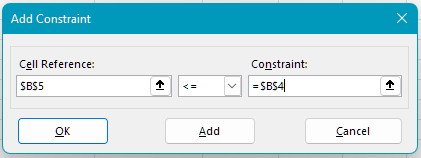
Click “Add,” and create two further constraints for sales of “Bottom” and “Top and Bottom” garments.
Click Add to create a constraint to only use whole numbers for sales. Add the data shown below:
Click “Add,” and create two further constraints for sales of “Top” and “Top and Bottom” garments.
Finally, click OK and the Solver window should look like this:
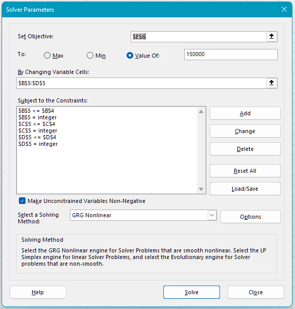
Click on “Solve.”
Solver tells you that it has found a solution. Click OK to keep Solver’s solution.
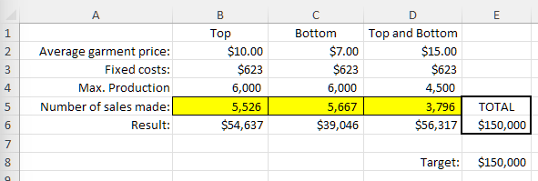
You’ll see that the yellow cells have now been populated, and the total is indeed $150,000! 😀
To obtain this figure while taking the constraints into account, Solver advises sales of 5526 “Top” garments, 5667 “Bottom” garments, and 3796 “Top and Bottom” garments.
Test Different Data Scenarios
Your boss and his colleagues are not sure how to price the different garments. Each of them has their own opinion on the average price for each garment category, and your boss asks you which price combination would be the most profitable for the business.
Here are the different price proposals:
Your boss’s proposal: $9 for tops, $8 for bottoms, and $14 for tops and bottoms
Tim’s proposal: $10 for tops, $7 for bottoms, and $15 for tops and bottoms
Rob’s proposal: $11 for tops, $8 for bottoms, and $13 for tops and bottoms
Excel can help you to create scenarios so you can compare the proposals! 😊
For this step, I’d advise you to download the scenarios file so that you can follow the demonstration below.
Prepare Your Scenario Analysis
Start by preparing the formula table which calculates the total number of sales:
Create Your Scenarios
Create Your Boss’s Scenario
Click on the “Data” tab, “What-If Analysis,” and then “Scenario Manager...”
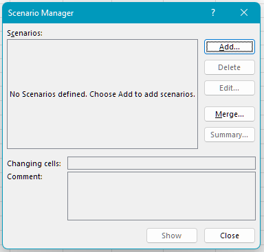
Click “Add...”
Name the first scenario “Boss’s opinion.”
Select the changing cells, in this case the yellow cells (
B2:D2).Click OK.
The changing cells window displays. Enter the first proposal.
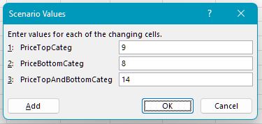
Click OK.
Create Tim’s Scenario
Repeat the above steps for the second scenario, with the average prices of $10 for tops, $7 for bottoms, and $15 for tops and bottoms.
Create Rob’s Scenario
Repeat the above steps for the third scenario, with the average prices of $11 for tops, $8 for bottoms, and $13 for tops and bottoms.
Compare the Different Scenarios
Click on the “Summary...” button.
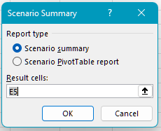
Select the cell containing the result formula (E5), then click on OK.
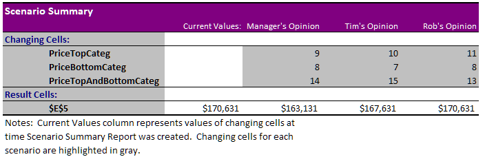
Ta-da! Excel creates a new tab, and completes its own comparison of the three proposals:
Over to You!
Download this file and do the following:
Use the Goal Seek feature to find the answer to problem 1 (green cell). The target is $75,000.
In problem 2, use Solver to achieve the $70,000 sales target, by playing around with the purchase price, the sales price, and the number of sales (orange cells).
Your constraints are:
The purchase price needs to be between $4 and $6.
The sales price needs to be between $22 and $26.
The minimum margin should be $20 or more.
Answer Key
Look at this file and watch the video below to check your work.
Let’s Recap!
Excel includes a range of analysis tools which you can use to solve complex problems.
You can use the Goal Seek tool to resolve problems with one unknown component.
You can use Solver to resolve complex problems with multiple constraints.
You can also use scenarios to compare different data sets.
Well done! You’ve just helped your boss to choose the best strategy! 🥳 Come with me to the next chapter to learn how to process large quantities of data.
